

 Open Access||Research Article
Target Circularity and Geographic Generalisation in Machine-Learning Prediction of a Water Quality Index: A Simulation-Based Methodological Critique for the Pra River Basin, Ghana
Frank B. K. Twenefour1,2 , Henry Otoo2, Eric Neebo Wiah2, Emmanuel Ayitey1
1 Department of Mathematics, Statistics and Actuarial Science, Faculty of Applied Science, Takoradi Technical University, P. O. Box 256, Takoradi, Western Region, Ghana
2 Department of Mathematical Science, Faculty of Engineering, University of Mines and Technology, P. O. Box 237, Tarkwa, Western Region, Ghana
Abstract
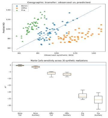
This methodological study uses a controlled simulation, not a new empirical assessment of Pra River Basin water quality, to examine two validation pitfalls that inflate apparent machine-learning performance in predicting a Water Quality Index (WQI): target circularity, where a model is scored on the variables used to construct the index, and optimistic within-domain validation, where random splits mask poor performance outside the sampled domain. A synthetic, 150-record benchmark was generated for the Birim, Offin and Pra sub-basins, with WQI calibrated as a near-deterministic function of pH, TSS, TDS and electrical conductivity. A full-feature model was compared with an auxiliary-only model using XGBoost, Random Forest, linear and Ridge regression, assessed via five-fold and leave-one-sub-basin-out validation. Full-feature XGBoost performed well within sub-basins (R² = 0.729–0.830) but dropped to negative R² when index-defining variables were removed. Transfer was weak for every model: XGBoost produced R² of 0.078 to 22.982 − − out-of-basin, and Ridge showed comparably negative transfer, confirming the failure was not confined to tree ensembles. Reduced auxiliary models did not recover transferable skill. Findings show strong local WQI prediction can coexist with poor geographic transfer and is not resolved by using linear rather than tree-based models, supporting validation aligned with intended deployment.
Keywords
Graphical Abstract
Novelty Statement
This study introduces a controlled simulation benchmark demonstrating how target circularity and optimistic within-domain validation mask catastrophic geographic transfer failures. The findings indicate that algorithmic complexity cannot substitute for spatial validation aligned with actual deployment conditions.
Graphical Abstract
1. Introduction
Water quality remains a central concern in environmental management because rivers and other surface-water systems support domestic supply, agriculture, fisheries, industry, ecosystem functioning and local livelihoods. The quality of these water resources is influenced by a combination of natural processes and anthropogenic activities, including erosion, sediment transport, land use change, wastewater discharge, agricultural runoff and mining-related disturbance.[1] In catchments where these pressures occur simultaneously, water quality may vary considerably over short distances and between connected subbasins. This spatial variability creates a practical challenge for monitoring programs because a limited number of sampling locations must represent environmental conditions that are often heterogeneous. As a result, there is growing interest in analytical methods that can support more efficient interpretation, prediction and prioritization of water quality information. Water quality indices (WQIs) are widely used for this purpose because they summarize several physicochemical measurements into a single value that is easier to communicate and compare across locations. [1-3] A WQI can be useful for describing broad differences in water conditions, identifying areas that may require closer attention and presenting complex monitoring information in a form that is accessible to decision makers. [1,2,4] Moreover, the usefulness of an index depends on how it is constructed. Its value is determined by the variables included, the standards applied to those variables and the weighting or aggregation procedure adopted.[1-3] Consequently, a WQI is not an independent environmental measurement; it is a derived quantity that reflects a defined combination of observed parameters. This characteristic becomes particularly important
when machine-learning methods are used to predict WQI values.
Machine learning has become increasingly prominent in water-quality research because it offers flexible tools for representing nonlinear associations, interactions and threshold behavior that may be difficult to capture using conventional regression models. Tree-based ensemble methods, including random forest and gradient boosting algorithms such as XGBoost, have been applied successfully to water quality prediction, water potability assessment and related environmental classification problems. More recent studies have also incorporated explainable artificial intelligence so that predictive performance can be accompanied by information on the relative contributions of individual variables.[5-9] These developments have strengthened the practical appeal of machine learning because users are increasingly interested not only in whether a model is accurate but also in why particular predictions are produced. Despite this progress, high predictive accuracy does not by itself demonstrate that a model is suitable for environmental decision-making. One important issue is the design of the validation procedure. Many machine learning studies use random training and test splits or conventional k-fold cross-validation. These procedures are useful for estimating internal predictive performance, but they can be optimistic when the observations are spatially structured. Samples drawn from the same catchment, monitoring network or hydrological unit may share similar environmental characteristics, which means that the test data may not be genuinely independent of the training domain. A model can therefore perform well because it is interpolating within a familiar environmental regime, while its ability to operate in a different location remains unknown.[4]
This problem is not specific to water-quality research: the broader ecological and environmental machine-learning literature has shown that random or nonblocked cross-validation systematically underestimates prediction error whenever data have temporal, spatial, hierarchical or phylogenetic structure and has recommended block- or domain-based cross-validation as a corrective.[10-12] Related work has formalized this concern as the “area of applicability” of a spatial prediction model—the region of predictor space on which the model was actually trained—and has shown that prediction quality decreases once new data fall outside that area, regardless of the learning algorithm used.[4] This distinction has become increasingly important in environmental machine learning, where generalization and transfer to unobserved sites are often more relevant than prediction within the original sample.[10-13] A related issue concerns the relationship between predictors and the response itself. When a composite index is predicted from the same variables used to calculate it, the task can become partly circular. In the Pra River Basin, the WQI is derived from the pH, total suspended solids (TSS), total dissolved solids (TDS) and electrical conductivity (EC); a model using these same variables can therefore achieve high accuracy by approximating the index-construction rule.[1] Such performance can be useful for automation or approximation, but it should not be interpreted as independent prediction or as evidence that the underlying field measurements can be replaced.[11,14] This dependence is better described as target circularity or index-component dependence than classical data leakage because the predictors may be legitimately available at the prediction time even if they are mathematically tied to the target.[11, 14] A rigorous assessment should therefore compare two settings: reconstruction when the index-defining variables are available and prediction from auxiliary variables alone. The second setting provides a stricter test of whether the model has learned relationships that may transfer beyond the index formulation.[11,15]
The Pra River Basin in Ghana provides an informative setting for examining these methodological issues. The basin system includes the Birim, Offin and Pra subbasins, whose WQI distributions differ substantially. Previous work using the same broader research program reported that the WQI was constructed from the pH, TSS, TDS and EC and that the three subbasins exhibited distinct water-quality regimes. A published geostatistical analysis further demonstrated meaningful spatial structure in WQI and revealed that ordinary kriging outperformed inverse distance weighting and cokriging for spatial interpolation across a 150-site monitoring network.[1] These findings indicate that water quality behavior in the basin is spatially organized rather than uniform, making the system appropriate for investigating whether relationships identified in one part of the basin can be transferred reliably to another. The same body of work also reported that many nutrient and trace-metal variables showed only weak individual linear associations with WQI.[1] This creates an analytically useful contrast. The variables used directly to calculate the WQI contain strong target-proximal information, whereas the auxiliary variables may represent broader environmental conditions without mathematically determining the index. A model that performs strongly with the direct WQI components but poorly with auxiliary variables would therefore suggest that the apparent predictive success depends largely on index reconstruction. Conversely, if auxiliary variables retain substantial predictive ability in an unseen subbasin, this would indicate the presence of more generalisable environmental information that could support screening or monitoring prioritization.[11,14]
Explainability is also relevant to this question. SHapley Additive exPlanations (SHAP) and permutation-based importance methods are being increasingly used to identify variables that influence machine-learning predictions.[11,16] SHAP assigns an importance value to each feature for a particular prediction, whereas permutation approaches assess how model performance changes when the information contained in a predictor is disrupted. However, variable importance should be interpreted in the context of model validity because explainability does not by itself demonstrate that a model has identified a robust or causal environmental relationship. A predictor may receive a high importance score in a model that generalizes poorly, particularly when the training data are limited, overfitted or unrepresentative of the intended prediction domain.[11,15] For this reason, explainability should be considered alongside rigorous out-of-sample or cross-domain validation rather than being treated as a substitute for predictive validity.[11] Comparing feature rankings across held-out subbasins therefore provides a useful means of assessing whether the model identifies relatively stable predictive relationships or whether the apparent importance of variables is specific to the environmental conditions represented during model development. These distinctions have direct monitoring implications. Machine learning may appear to reduce the measurement burden, but that claim is defensible only if useful performance persists when the direct WQI components are unavailable and when the model is applied outside its development domain.[1] A model that requires all index components may still assist rapid computation or quality control, but it does not reduce the underlying measurement requirement. Similarly, poor cross-subbasin performance limits claims of basin-wide deployment.
The present study is explicitly a methodological critique of machine-learning validation practices in hydrology and is examined through a case study built around the Pra River Basin rather than a new assessment of current water-quality conditions in the basin. It addresses this through a reproducible simulation informed by reported characteristics of the basin.[1] A synthetic design, rather than the existing field dataset, was chosen for three specific reasons. First, diagnosing target circularity and geographic transfer failure requires knowing the true data-generating relationship between the predictors and the response; with observational field data, the true functional form is unknown, so any transfer failure could be attributed either to a genuine methodological pitfall or to unmodeled environmental heterogeneity, and the two explanations cannot be separated. A simulation in which the WQI-generating rule is specified in advance removes this ambiguity: any degradation in cross-basin performance can be attributed to the validation design itself rather than to unexplained field variability. Second, a controlled benchmark allows the exact same underlying process to be regenerated under many independent random draws (the 30-replicate Monte Carlo design reported below), which is not possible with a single fixed field dataset and is necessary to show that the observed pattern is not an artifact of one particular sample. Third, this design keeps the present study clearly distinct from, and complementary to, the existing field-based geostatistical analysis of the same basin,[1] which already addresses spatial interpolation of observed WQI; the present study instead isolates a purely methodological question—how validation design and predictor definition affect apparent model performance—that a single observational dataset cannot answer in isolation. This study therefore does not introduce new field observations; it builds a 150-record benchmark that reproduces the previously reported WQI distributions and selected physicochemical characteristics for the Birim, Offin and Pra subbasins,[1,4] and any conclusions drawn are conclusions about the validation methodology, not about the present state of water quality in the basin. The full-feature and auxiliary-only models are compared, the within-subbasin and leave-one-subbasin-out performance is evaluated, the stability of feature importance is examined, a reduced-variable model is tested, whether the pattern is specific to tree-based learners is tested by adding linear and ridge regression, and the experiment is repeated across multiple independently generated datasets. The central objective is to determine whether strong local WQI prediction remains convincing when the analysis is subjected to stricter tests of target circularity and geographic generalization.[1,4] Accordingly, this study aims to evaluate the extent to which water quality index prediction is influenced by the inclusion of the variables used directly in the construction of the index and to determine whether the predictive relationships developed in the two subbasins can be transferred reliably to a third of the previously unseen subbasin. The analysis further examines whether the observed patterns are robust across model classes with fundamentally different extrapolation behaviors—the tree-based XGBoost and random forest learners, which partition rather than extrapolate the training range, and linear regression and ridge regression, which can in principle extrapolate linearly beyond it—to assess the stability of auxiliary variable importance across subbasins using SHAP and permutation importance and investigate whether a reduced set of auxiliary predictors can retain useful cross-subbasin predictive performance.
2. Materials and methods
2.1 Simulation framework and calibration targets
The analysis used a reproducible synthetic benchmark informed by summary statistics reported in the Pra River Basin research program, specifically the 150-station monitoring network and subbasin WQI statistics reported in Twenefour et al. (2026).[1,4] The benchmark contained 150 records, with 50 observations assigned to each of the Birim, Offin and Pra subbasins. The synthetic WQI distributions were calibrated to the basin means and standard deviations reported in that source, while the principal physicochemical variables were calibrated to the corresponding subbasin means.[1,4] As set out in the Introduction, this design was chosen specifically because it fixes the true data-generating relationship between predictors and WQI in advance, which is what allows target circularity and geographic-transfer failure to be attributed unambiguously to validation design rather than to unmodeled field heterogeneity. As shown in Table 1, the simulated WQI means and standard deviations closely reproduce the reported subbasin values. Methodologically, the purpose of this design was to examine model behavior under a data structure that resembled the reported basin system while retaining complete control over how the response and predictors were generated.
| Subbasin | n | Reported mean | Simulated mean | Reported SD | Simulated SD |
|---|---|---|---|---|---|
| Birim | 50 | 93.330 | 93.328 | 10.820 | 10.546 |
| Offin | 50 | 120.570 | 120.533 | 15.670 | 13.860 |
| Pra | 50 | 74.170 | 74.162 | 7.220 | 6.934 |
2.2 Data-generating procedure
The four variables used to define the WQI in the parent research program—pH, TSS, TDS and EC—were generated first. pH was simulated on an approximately normal scale, whereas TSS, TDS and EC were generated from log-normal distributions to preserve positivity and right-skewness. Moderate correlations were introduced among the suspended- and dissolved-load variables so that the simulated records did not behave as independent marginal samples. A WQI proxy was then generated from within-subbasin standardized values of the four index components using weights of 0.20 for pH, 0.30 for TSS, 0.25 for TDS and 0.25 for EC. A small random component was included to prevent perfectly deterministic mapping. The resulting values were rescaled to the reported mean and dispersion for each subbasin and constrained to the reported WQI range. The weighting rule was used only to construct a plausible simulation and is not presented as a reconstruction of the exact field-data WQI formula. The auxiliary variables included total nitrogen (TN), two phosphorus measures (TP1 and TP2), nitrate (NNO3), ammonium (NNH4), lead (Pb), mercury (Hg), arsenic (As), cadmium (Cd), copper (Cu) and iron (Fe). Their marginal distributions were generated on log-normal scales and calibrated to previously reported means and standard deviations. Weak associations with WQI were introduced using the direction and approximate magnitude of correlations reported in the doctoral analysis. Synthetic geographic coordinates were retained only as metadata and were not used in the primary prediction models. The reference simulation used the random seed 20260810. To determine whether the main conclusions were sensitive to one particular realization, the entire generation process was repeated independently 30 times using seeds 3001–3030.
2.3 Predictor sets
Three predictor settings were examined to separate index reconstruction from prediction based on independent auxiliary information. As detailed in Table 2, the full-feature model included the four variables used to construct the WQI together with all auxiliary measurements, whereas the auxiliary-only and reduced models excluded the direct WQI components.
| Model setting | Predictors | Purpose |
|---|---|---|
| Full-feature | pH, TSS, TDS, EC and all auxiliary variables | Benchmark that includes the variables defining WQI |
| Auxiliary-only | TN, TP1, TP2, NNO3, NNH4, Pb, Hg, As, Cd, Cu and Fe | Tests predictive information that is independent of the four WQI components |
| Reduced auxiliary | Four predictors selected from the training data | Tests whether a smaller predictor set improves portability |
2.4 Machine learning models
XGBoost was selected as the main regression algorithm because it can model nonlinear effects and interactions while remaining compatible with TreeSHAP explanations.[17] To keep the experiment focused on validation rather than extensive hyperparameter searching, a conservative specification was fixed in advance: maximum tree depth 2, learning rate 0.05, 250 boosting rounds, 0.90 row subsampling, 0.90 column subsampling, minimum child weight 3, L2 regularization 5 and L1 regularization 0.1. Random forest was used as a sensitivity model with 300 trees, square-root feature sampling and a minimum leaf size of 2.[18] It is important to note that fixed-depth tree ensembles cannot mathematically extrapolate beyond the range of target values observed during training. Consequently, a model failure under leave-one-subbasin-out cross-validation during an extreme hydrological regime—such as those observed in the Offin or Pra subbasins—could, in principle, reflect an inherent limitation of the learner class rather than a true shift in the underlying physical relationships. To test this possibility directly, ordinary least-squares linear regression and ridge regression (L₂ penalty, α = 1.0, with standardized predictors) were introduced as non-tree sensitivity baselines. Unlike XGBoost and random forest models, both linear frameworks possess the capacity to extrapolate outside the training bounds. This comparison provides a more rigorous evaluation of whether the downstream transfer failures reported herein are artifacts of tree-based partitioning or a broader systemic consequence of the simulation design.
2.5 Validation strategy
Two forms of validation were compared. The first used fivefold shuffled cross-validation separately within each subbasin. This represents a local prediction setting because training and validation observations come from the same simulated subbasin distribution. The second used leave-one-subbasin-out validation. As summarized in Table 3, each outer fold used two subbasins for model fitting and reserved the third subbasin entirely for testing.
| Fold | Training subbasins | Held-out subbasin |
|---|---|---|
| 1 | Offin + Pra | Birim |
| 2 | Birim + Pra | Offin |
| 3 | Birim + Offin | Pra |
2.6 Performance measures and uncertainty
Model performance was summarized using the root mean square error (RMSE), mean absolute error (MAE), coefficient of determination (R²), mean prediction bias, calibration intercept and calibration slope. For each held-out subbasin, 95% confidence intervals for the RMSE were estimated from 1,000 bootstrap resamples. To describe differences between the training and held-out domains, standardized mean differences and two-sample Kolmogorov–Smirnov statistics were calculated for the auxiliary variables. R² is reported throughout its general (nonintercept, out-of-sample) definition, R² = 1 - SSres/SStot, where SStot is computed from the held-out subbasin’s own mean. Under leave-one-subbasin-out validation, this quantity is not bounded below zero: A negative R² indicates that only the model’s predictions on the held-out subbasin were less accurate, in mean-square-error terms, than simply predicting that subbasin’s own mean WQI. This is a substantially stricter benchmark than the within-subbasin R² reported in Section 3.1, and the two quantities are not directly comparable; the negative values reported in Sections 3.2 to 3.6 should be read as “worse than the held-out mean,” not as a rescaled or bounded goodness-of-fit statistic.
2.7 Explainability and reduced-variable analysis
SHapley Additive exPlanations (SHAP) values were calculated from the auxiliary-only XGBoost model for each held-out subbasin.[16] The mean absolute SHAP values were used to rank the predictors, and the importance of permutation was calculated as an independent model-agnostic check. The stability of the SHAP ranks across subbasins was assessed with Spearman rank correlations. For the reduced-variable analysis, the four most important auxiliary predictors were selected using only the training data, and a new XGBoost model was fitted before evaluation on the held-out subbasin.
3. Results
3.1 Calibration and within-subbasin prediction
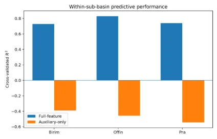
The reference simulation reproduced the intended WQI ordering across the three subbasins. The mean simulated WQI was 93.33 in Birim, 120.53 in Offin and 74.16 in Pra, closely matching the calibration targets reported in Table 1. Within each subbasin, XGBoost performed well when the four index components were available, as summarized in Table 4. As shown in Table 4, the full-feature model produced R² values of 0.729 for Birim, 0.830 for Offin and 0.739 for Pra. When the pH, TSS, TDS and EC were removed, the performance deteriorated sharply, with auxiliary-only R² values of -0.390, -0.457 and -0.545, respectively. The RMSE increased by 6.87 WQI units in Birim, 10.91 in Offin and 5.03 in Pra. This contrast is illustrated in Fig. 1, which shows a consistent reduction in predictive performance across all three subbasins. The results indicate that most of the local predictive strength in the simulated benchmark came from variables directly involved in constructing the WQI.
| Subbasin | Predictor setting | RMSE | MAE | R² | Bias |
|---|---|---|---|---|---|
| Birim | Full-feature | 5.436 | 4.362 | 0.729 | -0.477 |
| Birim | Auxiliary-only | 12.310 | 9.476 | -0.390 | 0.638 |
| Offin | Full-feature | 5.652 | 4.540 | 0.830 | 0.004 |
| Offin | Auxiliary-only | 16.560 | 13.567 | -0.457 | -0.321 |
| Pra | Full-feature | 3.506 | 2.649 | 0.739 | -0.567 |
| Pra | Auxiliary-only | 8.533 | 6.862 | -0.545 | -0.279 |
3.2 Cross-subbasin generalization
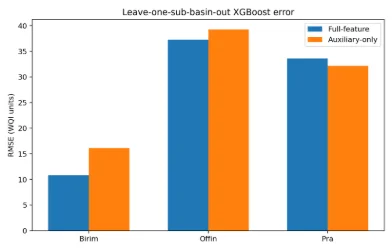
The results changed substantially when the model was transferred to a subbasin that was not represented during fitting. Table 5 presents the complete leave-one-subbasin-out results for XGBoost. For Birim, the full-feature model produced an RMSE of 10.838 and R² = -0.078, whereas the auxiliary-only model produced an RMSE of 16.118 and R² = -1.384. Transfer to Offin and Pra was substantially poorer. When Offin was held out,
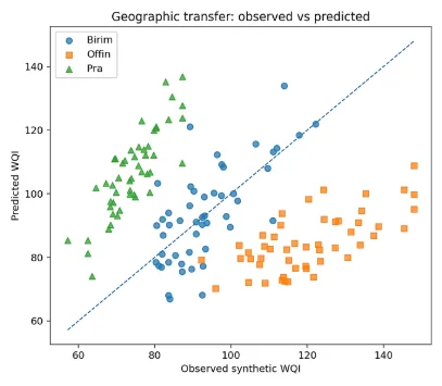
the full-feature model produced an RMSE of 37.289, R² = -6.386 and a bias of -35.854, indicating systematic underprediction of the high-WQI regime. When Pra was held out, the corresponding RMSE was 33.617 (R² = -22.982), and the bias was 32.538, indicating systematic overprediction of the low-WQI regime. These results show that the predictive relationships learned from the two subbasins did not generalize reliably to a third subbasin, indicating a substantially different WQI distribution. The increase in prediction error across the held-out subbasins is illustrated in Fig. 2. These results show that strong local prediction did not translate into reliable cross-subbasin extrapolation. Fig. 3 provides a complementary observed-versus-predicted view of the full-feature XGBoost model and shows the marked departure from the 1:1 line, particularly for the Offin and Pra holdout cases. This pattern is consistent with the response distributions used in the simulation: the training data for the Offin fold did not contain an equally high WQI regime, whereas the training data for the Pra fold did not contain an equally low regime.
| Held-out | Predictor setting | RMSE | 95% CI low | 95% CI high | MAE | R² | Bias |
|---|---|---|---|---|---|---|---|
| Birim | Full-feature | 10.838 | 8.376 | 13.188 | 8.251 | -0.078 | 0.410 |
| Birim | Auxiliary-only | 16.118 | 12.168 | 20.141 | 11.910 | -1.384 | 4.172 |
| Offin | Full-feature | 37.289 | 34.643 | 39.727 | 35.854 | -6.386 | -35.854 |
| Offin | Auxiliary-only | 39.246 | 34.894 | 43.401 | 35.533 | -7.181 | -35.245 |
| Pra | Full-feature | 33.617 | 31.280 | 36.000 | 32.538 | -22.982 | 32.538 |
| Pra | Auxiliary-only | 32.170 | 29.295 | 34.861 | 30.153 | -20.962 | 30.153 |
3.3 Sensitivity to model choice
Table 6 presents the random forest sensitivity results. Random forest improved the Birim transfer result under the full-feature setting (R²=0.522), but it did not change the broader conclusion. The performance remained poor when Offin (R²=-6.628) and Pra (R²=-21.933) were held out, and the auxiliary-only random forest models failed in all three folds. The lack of transferability was therefore not confined to a single-ensemble method.
| Held-out | Predictor setting | RMSE | MAE | R² | Bias |
|---|---|---|---|---|---|
| Birim | Full-feature | 7.219 | 5.938 | 0.522 | 2.555 |
| Birim | Auxiliary-only | 12.877 | 10.623 | -0.521 | 4.706 |
| Offin | Full-feature | 37.894 | 36.394 | -6.628 | -36.394 |
| Offin | Auxiliary-only | 38.728 | 35.844 | -6.967 | -35.844 |
| Pra | Full-feature | 32.873 | 32.715 | -21.933 | 32.715 |
| Pra | Auxiliary-only | 32.987 | 31.954 | -22.091 | 31.954 |
3.3.1 Nontree sensitivity models: linear regression and ridge regression
To evaluate model performance against non-tree baselines, ordinary least-squares linear regression and ridge regression were fitted to the same leave-one-subbasin-out cross-validation folds using the identical predictor configurations detailed in Tables 5 and 6. Table 7 reports the reference-seed results, alongside a 30-replicate Monte Carlo summary for the ridge regression models evaluated on independently regenerated benchmarks under the uniform experimental design described in Section 2.2.
| Held-out | Model | Predictor setting | RMSE | R² | Median R² (30-rep MC, Ridge) |
|---|---|---|---|---|---|
| Birim | Ridge regression | Full-feature | 7.11 | 0.489 | 0.008 (IQR -1.48 to 0.61) |
| Birim | Ridge regression | Auxiliary-only | 12.51 | -0.583 | -4.83 (IQR -12.03 to -1.06) |
| Offin | Ridge regression | Full-feature | 29.18 | -4.753 | -0.068 (IQR -0.50 to 0.21) |
| Offin | Ridge regression | Auxiliary-only | 102.10 | -69.437 | -7.61 (IQR -13.10 to -3.29) |
| Pra | Ridge regression | Full-feature | 10.23 | -1.248 | -5.79 (IQR -11.10 to -3.17) |
| Pra | Ridge regression | Auxiliary-only | 30.51 | -19.003 | -30.52 (IQR -54.56 to -18.11) |
| Birim | Linear regression | Full-feature | 7.37 | 0.451 | – |
| Offin | Linear regression | Full-feature | 28.68 | -4.557 | – |
| Pra | Linear regression | Full-feature | 10.38 | -1.313 | – |
As Table 7 shows, replacing the tree-based learners with linear regression or ridge regression did not restore reliable geographic transfer: full-feature transfer R² remained negative for Offin and Pra under both linear methods and across the Monte Carlo replicates, and the auxiliary-only Ridge model transferred especially poorly to Offin (median R² = -7.61, with individual replicates as low as R² = -69 at the reference seed) because unconstrained linear extrapolation of noisy, weakly associated auxiliary predictors far outside their training range can overshoot more severely than a tree-based model, which cannot predict outside the range of values seen in training. Linear and ridge regression therefore did not resolve, and in the auxiliary-only setting could worsen, the geographic-transfer problem identified with XGBoost and random forest.
The structural reason for these results follows directly from the data-generating design described in Section 2.2: because the WQI was constructed from within-subbasin standardized values of pH, TSS, TDS, and EC, the mapping from raw predictor values to the WQI is, by construction, defined using different standardization constants (means and standard deviations) in each subbasin. The “true” functional relationship between the raw predictors and the target therefore differs across subbasins by design. Consequently, no fixed global model—tree-based or linear—can, in principle, reproduce all three subbasin relationships simultaneously when trained on only two of them. This clarifies why the introduction of the non-tree baseline models, while serving as a necessary and informative sensitivity check, does not by itself resolve the transfer problem: the limitation demonstrated here is not an artifact of tree-based extrapolation, but rather a structural consequence of how the simulated WQI response was defined.
3.4 Feature importance across held-out subbasins
The leading auxiliary variables for each held-out subbasin are reported in Table 8. NNO3, TP2, As, NNH4 and Cd were the five highest-ranked variables when Birim was held out. For Offin, the leading variables were NNH4, Cu, Pb, Fe and TP1, whereas the NNO3, As, Hg, TP1 and TP2 were the most highly ranked in the Pra model. The average mean absolute SHAP importance across the three holdout settings is summarized in Fig. 4. The pairwise Spearman correlations between the SHAP rankings were -0.409 for Birim versus Offin, 0.573 for Birim versus Pra and -0.455 for Offin versus Pra. The low and inconsistent rank correlations indicate that a single basin-wide importance ordering would not be well supported by this simulation.
| Held-out | Rank | Variable | Mean |SHAP| |
|---|---|---|---|
| Birim | 1 | NNO3 | 5.526 |
| Birim | 2 | TP2 | 5.090 |
| Birim | 3 | AS | 3.981 |
| Birim | 4 | NNH4 | 3.452 |
| Birim | 5 | CD | 3.210 |
| Offin | 1 | NNH4 | 3.289 |
| Offin | 2 | CU | 2.418 |
| Offin | 3 | PB | 2.059 |
| Offin | 4 | FE | 1.526 |
| Offin | 5 | TP1 | 1.205 |
| Pra | 1 | NNO3 | 4.369 |
| Pra | 2 | AS | 2.644 |
| Pra | 3 | HG | 2.408 |
| Pra | 4 | TP1 | 1.892 |
| Pra | 5 | TP2 | 1.869 |
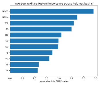
By design, the auxiliary variables were calibrated with only weak, basin-specific associations with the WQI (Section 2.2); thus, two distinct mechanisms can, in principle, produce this instability: (i) a genuine domain or covariate shift, in which the direction or strength of an auxiliary variable’s relationship with the WQI differs across subbasins, mirroring the way the WQI-generating rule itself is defined per subbasin (Section 3.3.1); and (ii) a low signal-to-noise ratio, in which weak correlations make the SHAP rankings sensitive to sampling variation even when the underlying association is broadly stable. The reference simulation cannot fully separate these two mechanisms because the auxiliary-variable correlations were themselves generated with basin-specific direction and magnitude, which builds a form of domain shift directly into the data. What can be said from the design is that the instability is not attributable to the auxiliary variables carrying strong, basin-invariant signals that SHAP failed to detect: their weak calibrated correlations mean that even a correctly specified model has limited auxiliary-variable information to rank consistently. In practice, this means that SHAP rankings from a single subbasin should not be read as evidence of a basin-wide environmental driver without corroborating evidence from an independent subbasin.
3.5 Reduced auxiliary models
The data in Table 9 indicate that reducing the number of auxiliary predictors did not improve cross-subbasin performance. The reduced models produced R²=-2.795 for Birim, -7.581 for Offin and -23.859 for Pra. The selected variables also changed across the three training folds, which is consistent with the instability observed in the SHAP rankings reported in Table 8.
| Held-out | Training-selected variables | RMSE | R² | Bias |
|---|---|---|---|---|
| Birim | TP2, CU, NNO3, AS | 20.337 | -2.795 | 3.888 |
| Offin | NNH4, CU, PB, FE | 40.192 | -7.581 | -36.027 |
| Pra | HG, NNO3, CD, CU | 34.226 | -23.859 | 31.902 |
3.6 Monte Carlo sensitivity
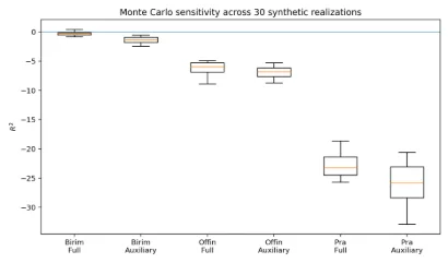
The Monte Carlo results are summarized in Table 10. The 30-replicate experiment revealed that the reference results were not an isolated consequence of one random seed. For the full-feature XGBoost model, the median transfer R² was -0.231 for Birim, -5.968 for Offin and -23.247 for Pra. The auxiliary-only models remained weaker. The distribution of R² values across the 30 independent simulation replicates is shown in Fig. 5, which confirms that the transfer pattern persisted across repeated datasets rather than being driven by a single generated sample. Overall, the local structure could be learned, but extrapolation to an unseen subbasin remained unreliable.
| Held-out | Predictor setting | Median RMSE | RMSE Q1 | RMSE Q3 | Median R² | R² Q1 | R² Q3 |
|---|---|---|---|---|---|---|---|
| Birim | Auxiliary-only | 15.963 | 14.840 | 16.719 | -1.311 | -1.790 | -0.944 |
| Birim | Full-feature | 11.554 | 11.112 | 12.585 | -0.231 | -0.531 | -0.109 |
| Offin | Auxiliary-only | 39.235 | 38.253 | 40.030 | -6.829 | -7.619 | -6.142 |
| Offin | Full-feature | 37.103 | 36.697 | 37.904 | -5.968 | -6.839 | -5.242 |
| Pra | Auxiliary-only | 33.563 | 32.379 | 34.874 | -25.860 | -28.365 | -23.090 |
| Pra | Full-feature | 31.850 | 31.460 | 32.501 | -23.247 | -24.460 | -21.342 |
4. Discussion
The main finding is the contrast between local model accuracy and geographic transfer. In the simulated data, full-feature XGBoost explained approximately 73–83% of the WQI variation when validation remained within the same subbasin. That level of performance would ordinarily be regarded as strong. The picture changed, however, when the model was asked to predict an unseen subbasin. The transfer performance fell below the mean-prediction benchmark in all three XGBoost folds and was particularly poor for Offin and Pra. These results illustrate why environmental model evaluation should be tied to the intended prediction setting rather than be based solely on random or within-domain validation.[10,11] A second result concerns the role of the variables used to construct the WQI. Removing the pH, TSS, TDS and EC eliminated the strong within-subbasin performance. This drop is an expected, designed artifact of the simulation rather than a novel empirical finding: because the synthetic WQI was constructed as a near-deterministic weighted combination of exactly these four variables plus a small noise term (Section 2.2), a model without them has, by construction, been deprived of almost all of the information that determines the target, and a sharp decline in auxiliary-only R² is the anticipated consequence of that design rather than evidence of anything unexpected about auxiliary water-quality variables in general. Nonetheless, the results have important methodological implications for applied studies working with real field data, where this deterministic structure is not known in advance: When an index is predicted from its own component variables, the resulting accuracy should be interpreted primarily as index reconstruction unless the study also demonstrates useful performance from independent information. Such a distinction is particularly important when machine learning is proposed as a way to reduce field or laboratory measurements.
The transfer results for Offin and Pra also highlight the difficulty of extrapolation with tree-based models. Both XGBoost and random forest are effective at partitioning the range of predictor‒response relationships represented in the training data, but neither is naturally suited to extrapolating far beyond that range. In the present simulation, Offin occupied the upper end of the WQI distribution, and Pra occupied the lower end. When either extreme regime was absent from the training set, predictions were pulled toward the range represented by the remaining two subbasins. However, the additional linear regression and ridge regression analysis (Section 3.3.1), conducted specifically to test this explanation, revealed that replacing the tree ensembles with models capable of linear extrapolation did not resolve the transfer failure and, for the auxiliary-only setting, could produce even more extreme errors than the tree-based models did. This finding indicates that the poor cross-subbasin transfer observed here reflects the basin-specific way the simulated response was constructed (Section 3.3.1) at least as much as it reflects any particular learning algorithm’s extrapolation behavior, which is consistent with the broader finding in the spatial prediction literature that transfer failure outside a model’s area of applicability is a general property of the training–test relationship rather than of any one algorithm.[4,12,13] The explainability analysis reinforces the same caution. SHAP is valuable for describing how a fitted model uses its predictors, and its use in water-quality studies has expanded rapidly.[6-9] However, a feature can be important to a model that generalizes poorly. Here, the leading auxiliary variables varied considerably across held-out subbasins, and the rank correlations were weak or negative for the two basin pairs. The explanation therefore depended on the geographic context. The reduced-variable models did not provide evidence that a small set of auxiliary variables could replace the index components. Their performance remained poor, and the selected features differed across folds. In practical terms, this means that feature importance rankings should not be translated directly into a reduced monitoring program without first demonstrating that the reduced model performs adequately in independent locations.
5. Conclusion
In this study, a Pra-informed simulation with a fully known and deliberately deterministic ground truth is used to examine whether strong local WQI prediction persists under stricter forms of validation. The full-feature XGBoost models performed well when training and validation observations came from the same subbasin, but the apparent advantage largely disappeared when the four WQI-defining variables were excluded—an expected consequence of the simulation design rather than a novel finding in itself. More importantly, the prediction deteriorated sharply when the models were transferred to an unseen subbasin, particularly when the held-out basin represented a WQI regime not present in the training data. Random forest produced the same broad pattern. Furthermore, linear regression and ridge regression, which can extrapolate linearly beyond the training range, produced the same qualitative failure to transfer; in the auxiliary-only setting, these linear models occasionally underperformed compared to their tree-based counterparts. This finding shows that the transfer failure documented here is tied to how the simulated response was constructed on a subbasin-specific basis rather than being an artifact specific to tree-based learners. SHAP rankings were geographically unstable, which is consistent with the deliberately weak and basin-specific auxiliary-variable correlations built into the simulation, and the reduced auxiliary models did not restore transferable skill.
Acknowledgements
Not applicable.
Funding Declaration
This research did not receive any specific grant from funding agencies in the public, commercial, or not-for-profit sectors.
Data Availability Statement
The datasets generated and analyzed during the current study (the synthetic benchmark, generation seeds, model specifications and calibration procedures) are not publicly available in a repository at the time of submission but are available from the corresponding author upon reasonable request.
Conflict of Interest
There is no conflict of interest.
Artificial Intelligence (AI) Use Disclosure
The authors declare that artificial intelligence (AI)-assisted tools were used only for language refinement, grammar improvement, and manuscript structuring purposes during the preparation of this work. All technical content, experimental implementation, results, and interpretations were independently developed and verified by the authors.
Supporting Information
Supporting Information
References
- [01] F. B. K. Twenefour, H. Otoo, E. N. Wiah, E. Ayitey, Spatial trend and geostatistical prediction of Water Quality Index in the Pra River Basin of Ghana, International Journal of Environment and Climate Change, 2026, 16, 129–140, 10.9734/ijecc/2026/v16i75528
- [02] M. G. Uddin, S. Nash, A. I. Olbert, A review of water quality index models and their use for assessing surface water quality, Ecological Indicators, 2021, 122, 107218, 10.1016/j.ecolind.2020.107218
- [03] M. Kachroud, F. Troland, M. Kefi, S. Jeberi, G. Bourrié, Water quality indices: Challenges and application limits in the literature, Water, 2019, 11, 361, 10.3390/w11020361
- [04] F. B. K. Twenefour, H. Otoo, E. N. Wiah, Robust inference and management prioritization of subbasin water-quality heterogeneity in the Pra River Basin, Ghana, Asian Journal of Geographical Research, 2026, 9, 11-18, 10.9734/ajgr/2026/v9i4460
- [05] A. Aldrees, M. Khan, A. T. B. Taha, M. Ali, Evaluation of water quality indices with novel machine learning and SHapley Additive ExPlanation (SHAP) approaches, Journal of Water Process Engineering, 2024, 58, 104789, 10.1016/j.jwpe.2024.104789
- [06] R. K. Makumbura, L. Mampitiya, N. Rathnayake, D. P. P. Meddage, S. Henna, T. L. Dang, Y. Hoshino, U. Rathnayake, Advancing water quality assessment and prediction using machine learning models, coupled with explainable artificial intelligence techniques like SHapley Additive ExPlanations (SHAP) for interpreting the black-box nature, The results in Engineering, 2024, 23, 102831, 10.1016/j.rineng.2024.102831
- [07] M. K. Nallakaruppan, E. Gangadevi, M. L. Shri, B. Balusamy, S. Bhattacharya, S. Selvarajan, Reliable water quality prediction and parametric analysis using explainable AI models, Scientific Reports, 2024, 14, 7520, 10.1038/s41598-024-56775-y
- [08] R. Choudhary, A. Kumar, C. Priyadharsini, M. M. Naik, M. Choudhury, N. A. Khan, Predicting water quality index using stacked ensemble regression and SHAP based explainable artificial intelligence, Scientific Reports, 2025, 15, 31139, 10.1038/s41598-025-09463-4
- [09] W. Li, M. Deng, C. Liu, Q. Cao, Analysis of key influencing factors of water quality in Tai Lake Basin based on XGBoost-SHAP, Water, 2025, 17, 1619, 10.3390/w17111619
- [10] A. Elahi, D. Shumway, M. Kowalcyk, A. Shrestha, D. Caragea, C. Caragea, S. Dorevitch, Machine learning, generalization, and transfer learning for predicting the exceedance of fecal indicator bacteria thresholds at beaches, Environmental Science & Technology, 2025, 59, 22386–22396, 10.1021/acs.est.5c02835
- [11] Z. Yan, J. Li, W. Zhang, H. Wen, H. Yu, M. Yu, Q. Liu, G. Jiang, A tutorial on best practices and pitfalls in applying machine learning to environmental research, ACS Environmental Au, 2026, 6, 553–565, 10.1021/acsenvironau.6c00025
- [12] D. R. Roberts, V. Bahn, S. Ciuti, M. S. Boyce, J. Elith, G. Guillera-Arroita, S. Hauenstein, J. J. Lahoz-Monfort, B. Schröder, W. Thuiller, D. I. Warton, B. A. Wintle, F. Hartig, C. F. Dormann, Cross-validation strategies for data with temporal, spatial, hierarchical, or phylogenetic structure, Ecography, 2017, 40, 913–929, 10.1111/ecog.02881
- [13] H. Meyer, E. Pebesma, E, Predicting into unknown space? Estimating the area of applicability of spatial prediction models, Methods in Ecology and Evolution, 2021, 12, 1620–1633, 10.1111/2041-210X.13650
- [14] S. Kapoor, A. Narayanan, Leakage and the reproducibility crisis in machine-learning-based science, Patterns, 2023, 4, 100804, 10.1016/j.patter.2023.100804
- [15] J. J. Zhu, M. Yang, Z. J. Ren, Machine learning in environmental research: Common pitfalls and best practices, Environmental Science & Technology, 2023, 57, 17671–17689, 10.1021/acs.est.3c00026
- [16] S. M. Lundberg, S. I. Lee, A unified approach to interpreting model predictions, 31st Conference on Neural Information Processing Systems, Long Beach, CA, USA, 2017.
- [17] T. Chen, C. Guestrin, XGBoost: A scalable tree boosting system, Proceedings of the 22nd ACM SIGKDD International Conference on Knowledge Discovery and Data Mining, Association for Computing Machinery, New York, NY, United States, 2016, 785–794. 10.1145/2939672.2939785
- [18] L. Breiman, Random forests, Machine Learning, 2001, 45, 5–32, 10.1023/A:1010933404324
Publisher Note
Publisher Note: The views, statements, and data in all publications solely belong to the authors and contributors. GR Scholastic is not responsible for any injury resulting from the ideas, methods, or products mentioned. GR Scholastic remains neutral regarding jurisdictional claims in published maps and institutional affiliations.
Open Access
This article is licensed under a Creative Commons Attribution-NonCommercial 4.0 International License, which permits the non-commercial use, sharing, adaptation, distribution and reproduction in any medium or format, as long as appropriate credit to the original author(s) and the source is given by providing a link to the Creative Commons License and changes need to be indicated if there are any. The images or other third-party material in this article are included in the article's Creative Commons License, unless indicated otherwise in a credit line to the material. If material is not included in the article's Creative Commons License and your intended use is not permitted by statutory regulation or exceeds the permitted use, you will need to obtain permission directly from the copyright holder. To view a copy of this License, visit: https://creativecommons.org/licenses/by-nc/4.0/
© The Author(s) 2026