

 Open Access||Research Article
A Comparative Study on the Thermal Performance of Copper and Stainless-Steel Heat Pipes
Karthik Tummalapalli1 , Sahil Wagh1, Hardik Dhumal1, Omkar Batwale1, Vishal Kandalgaonkar1
Department of Mechanical & Automation Engineering, Pravin Rohidas Patil College of Engineering & Technology, Mahavidyalaya Marg, Navghar, Bhayandar (East), Thane, Maharashtra, 401105, India
Abstract
Heat pipes are highly efficient passive thermal devices that exploit phase-change mechanisms —evaporation and condensation of a working fluid—to transport heat with minimal temperature drop. This study presents an experimental and computational investigation of a 204 mm copper–water heat pipe equipped with a stainless-steel mesh wick for small-scale thermal management. Steady-state temperature distribution, thermal resistance, heat-transfer rate, phase-change characterization, structural deformation, and stress distribution were evaluated under controlled laboratory conditions. ANSYS steady-state thermal simulations were performed to reproduce the measured temperature distribution as a conduction-only, single-phase representation of the solid wall; the model does not resolve two-phase vapor–liquid transport within the wick. A material comparison between copper and stainless steel 304 (SS304) was conducted under identical geometric and boundary conditions with only the wall thermal conductivity varied; all the SS304 results were analytical/numerical estimates and were not independently validated by experiments (see Limitations). The copper heat pipe achieved a conduction-based heat-transfer rate of 31.15 W (analytically derived from the measured evaporator–condenser temperature difference), a thermal resistance of 1.605 K/W, and a minimum vapor mass flow rate of 1.35 × 10⁻⁵ kg/s. In contrast, the SS304 equivalent yielded 1.17 W and 42.4 K/W, demonstrating the severe impact of low wall conductivity on heat-pipe performance under this scaling approach. The ANSYS contours were consistent with smooth heat spreading in copper and a steep gradient in SS304, with the simulated copper ΔT (≈ 43 K) within 14% of the measured value (50 K; see Section 4.6.1). These findings are consistent with the superiority of copper–water systems for compact, high-performance thermal management under the tested conditions.
Keywords
Graphical Abstract
Novelty Statement
This study combines laboratory experimentation, ANSYS steady-state simulation, and analytical material comparison within a unified framework to quantify the impact of pipe-wall conductivity on heat-pipe performance. The explicit documentation of ANSYS boundary conditions, inclusion of phase-change heat transfer characterization via latent heat analysis, and clear delineation between experimental copper data and analytically derived stainless-steel results provide a reproducible benchmark for material selection in compact thermal management systems.
1. Introduction
Efficient thermal management has become increasingly important in modern engineering systems such as consumer electronics, renewable-energy equipment, aerospace platforms, and industrial heat-recovery systems.[1,2] Conventional cooling approaches can become less attractive when high heat fluxes must be handled within compact geometries. Heat pipes address this requirement by using evaporation and condensation of a working fluid to transport heat with a small temperature difference and without mechanical pumping.[1,2] A conventional heat pipe comprises an evaporator, an adiabatic section, and a condenser; a wick returns the condensed liquid to the evaporator through capillary action.[1] The present study investigates a copper–water heat pipe experimentally and uses a single-phase ANSYS conduction model to reproduce the measured wall-temperature field. An analytical extension to SS304 is then used to examine the sensitivity of the calculated performance to wall thermal conductivity, while explicitly treating the SS304 case as an unvalidated analytical/numerical estimate.
2. Literature Review
Faghri describes heat pipes as passive two-phase thermal devices in which evaporation, vapor transport, condensation, and capillary liquid return enable heat transport with small temperature differences.[1] Vasiliev reviews heat-pipe applications in thermal management and heat-exchanger systems and emphasizes the importance of wick and operating conditions.[2] Mahdavi et al. experimentally investigated a cylindrical copper–water heat pipe with screen-mesh wick and examined the effects of heat input, inclination angle, and working-fluid fill volume.[3] Kempers et al. characterized the evaporator and condenser thermal resistances of a copper–water heat pipe with screen-mesh wick and showed that the heat-transfer mechanisms can include conduction and boiling in the evaporator.[4] Putra et al. demonstrated experimentally that screen-mesh wick structure influences the thermal resistance and performance of heat pipes.[5] Wang and Wan showed that stainless-steel heat pipes with sintered stainless-steel fiber wicks can achieve useful thermal performance when wick geometry and working-fluid wettability are considered.[6] Reddy et al. used response-surface modelling to show that heat load, tilt angle, and working-fluid formulation interact strongly in screen-mesh wick heat pipes.[7] De Araújo et al. experimentally demonstrated a water–stainless-steel rod-plate heat pipe with low measured thermal resistance when the device geometry and wick design were purpose-built for stainless steel.[8] Mansouri et al. and Xin et al. investigated grooved and wick-optimized copper flat heat pipes, illustrating the influence of wick geometry on thermal performance.[9,10] Scigliano et al. applied an ANSYS-based numerical framework to heat-pipe thermal performance for aerospace cooling.[11] Saad et al. showed that heat input and filling-fluid charge affect miniature heat-pipe performance, while Wong and Deng demonstrated that composite mesh–groove–powder wick architectures can significantly affect heat-transfer capability.[12,13] Sanhan et al. further showed experimentally and numerically that flattening and bending can alter miniature heat-pipe thermal performance.[14] Solomon et al. also demonstrated numerically that screen-mesh wick structure and working-fluid properties affect the predicted thermal field and heat-transfer behaviour.[15] These studies indicate that wall material is only one of several factors governing heat-pipe performance; wick structure, working-fluid charge, geometry, orientation, and operating conditions must also be considered. The present SS304 comparison therefore remains deliberately limited to a wall-conductivity-only analytical scaling.
3. Methodology
3.1 Heat pipe specifications
The test article was a commercially available copper heat pipe with the following specifications:
- Length: 204 mm
- Outer diameter: 22.5 mm; inner diameter: 20.5 mm; wall thickness: 1.0 mm
- Pipe material: Copper (thermal conductivity k = 400 W/m·K)
- Wick: Stainless steel wire mesh, SS304, plain weave, 200 mesh, 0.050 mm wire diameter (commercial product listing, GSR India via aajjo.com). The supplier's specification sheet does not state porosity, permeability, or wick thickness, and these remain unavailable for this batch (see Limitations, Section 5); the 200-mesh, 0.050 mm-wire specification is consistent with the fine woven meshes typically used as capillary wicks in heat pipes.
- Working fluid: Distilled water, 50 mL fill volume (≈74% of the internal pipe volume, V = πD²innerL/4 ≈ 67.3 mL; the fill was set to leave an adequate vapor-core volume while fully wetting the wick at startup)
- Evaporator heating: Low-intensity LPG flame (single-burner butane–propane torch, needle valve throttled to a low, visually steady flame; heat input was not independently metered—see Limitations)
- Condenser cooling: Hair dryer in cold-air mode (h ≈ 25 W/m²·K, within the 10–100 W/m²·K range typical of low-velocity forced-air convection over a cylindrical surface; taken as a representative estimate rather than a measured value — see Limitations)
- Adiabatic section insulation: Cotton wadding wrapped in aluminum foil
3.2 Methodology flowchart
Fig. 1 shows methodology flowchart showing the nine sequential steps of the study: from heat-pipe selection and test-setup preparation through sensor installation, system stabilisation, data recording, heat-transfer analysis, results comparison, and conclusions.
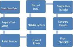
Fig. 1: Methodological workflow for experimental heat-pipe performance evaluation.
3.3 Experimental procedure
The heat pipe was positioned horizontally during testing to ensure a uniform liquid distribution along the wick and to eliminate gravitational bias in the condensate return (Fig. 2).[5] The evaporator was heated using a controlled low-intensity LPG burner, providing steady and reproducible heat input. The condenser was cooled by forced convection using a hair dryer in cold-air mode.[1,2] The adiabatic section was wrapped with cotton wadding and aluminum foil to minimize parasitic heat loss.[2] Temperature readings were recorded using three calibrated digital probe thermometers (SOLARA Digital LCD Cooking Food Thermometer, stainless-steel probe; manufacturer-stated accuracy ±1 °C), each checked against an ice-water bath (0 °C reference) before testing. The three sensors were positioned at the evaporator, at the mid-length of the adiabatic section, and at the condenser, with readings logged at 30-second intervals. Heating was applied gradually until a steady state was achieved (no further change in evaporator temperature over a 2-minute window), followed by removal of the heat source to observe the cooling cycle. The following parameters were monitored:
- Temperature rise at the evaporator
- Temperature at the mid-length adiabatic section
- Time delay in the condenser temperature response
- Cooling-cycle behavior after heat-source removal
- Visual confirmation of condensation on the condenser outer surface
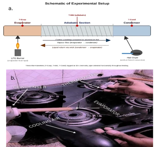
Fig. 2: (a) Schematic of the experimental setup, showing the evaporator (LPG burner), adiabatic section (cotton/aluminum-foil insulation), and condenser (hair dryer, cold-air mode), with the three thermometer locations and the direction of vapor flow and wick liquid return. (b) Photograph of the experimental setup: LPG burner at the evaporator end (right), cotton-and-aluminum-foil insulation on the adiabatic section (center), and a hair dryer providing cold-air forced convection at the condenser end (left).
The test was repeated three times under nominally identical conditions. The reported evaporator/condenser temperatures and derived quantities (Q, Rth, keff) are the averages of these three trials; the readings were consistent across all three runs to within the ±1 °C instrument resolution, with no additional scatter observed beyond this (see Section 4.7 for the propagated uncertainty).
3.4 Experimental setup
The evaporator was heated using a controlled low-intensity LPG burner, providing steady and reproducible heat input. The condenser was cooled by forced convection using a hair dryer in cold-air mode. The adiabatic section was wrapped with cotton wadding and aluminum foil to minimize parasitic heat loss (Fig. 2). A labeled schematic of the setup is shown in Fig. 2a, and the physical test rig is shown in Fig. 2b. Three digital thermometers were placed at the evaporator, mid-length adiabatic section, and condenser (Section 3.2). During heating, the evaporator temperature sharply increased, confirming active vapor formation. The condenser temperature increased more gradually, reflecting vapor transport and condensation.[1] Once the heat source was removed, the pipe cooled rapidly, confirming efficient redistribution of the condensate via the wick.[5]
3.5 ANSYS simulation setup
ANSYS steady-state thermal analysis was performed to (i) reproduce the experimental temperature distribution for the copper heat pipe as a conduction-only, single-phase solid-wall model and (ii) simulate the stainless-steel scenario under identical boundary conditions with only the wall thermal conductivity changed to 15 W/m·K.
3.5.1 Governing assumptions
- Steady-state conditions apply; all thermal quantities are time-invariant at the simulated operating point.
- Pipe wall material is homogeneous and isotropic with temperature-independent thermal conductivity (copper: 400 W/m·K; SS304: 15 W/m·K).
- The wick and working fluid are represented as effective thermal media; detailed two-phase flow within the wick is not resolved—the model is a solid-conduction representation only, and simulated temperature fields should be read as thermal-field validation under the prescribed boundary conditions rather than as direct evidence of evaporation, condensation, vapor transport, or wick liquid return.
- The dominant modeling mechanism in the solid wall is conduction; the evaporation–condensation contribution is characterized separately via latent heat analysis (Section 4.3).
- Radiation heat loss from the outer pipe surface is neglected.
- The adiabatic section outer wall is treated as perfectly insulated (zero heat flux).
3.5.2 Mesh
The solid-body geometry was meshed in ANSYS Workbench using program-controlled default sizing (no manual mesh refinement or element-count study was performed). No mesh-independence study was carried out; given the simple axisymmetric solid geometry and steady-state conduction-only physics, the mesh sensitivity is expected to be low, but this has not been formally verified and is listed as a limitation (Section 5).
3.5.3 Applied boundary conditions
The evaporator boundary condition was applied as a uniform heat flux q″ = Q/Aevap over the evaporator outer surface (Aevap = πDouterℓe, where ℓe is the evaporator section length). For copper, Q = 31.15 W; for SS304, Q = 1.17 W—both analytically derived from the measured evaporator–condenser temperature difference (Section 4.2) and not independently measured heat inputs (see also Section 4.6.1 and Limitations for the consequences of this for the ANSYS "validation"). The condenser boundary condition was applied as a convective condition, q″ = h(Twall − T∞), with h = 25 W/m²·K and T∞ = 30 °C, which is identical for both materials since the condenser cooling method (hair dryer, cold-air mode) did not change between simulations.
The complete boundary condition set for each material is summarized below:
Copper simulation
- Evaporator outer surface: uniform heat flux q″ = Q/Aevap, with Q = 31.15 W.
- Condenser outer surface: convective cooling, h = 25 W/m²·K, T∞ = 30 °C.
- Adiabatic section outer wall: zero heat flux (adiabatic boundary), representing the cotton/aluminum-foil insulation.
- All remaining surfaces: adiabatic (insulated).
- The wall material is copper, k = 400 W/m·K (isotropic, temperature independent).
SS304 simulation
- Evaporator outer surface: uniform heat flux q″ = Q/Aevap, with Q = 1.17 W (scaled per Section 4.5—not an independently measured or independently simulated heat input for a real SS304 unit).
- Condenser outer surface: convective cooling, h = 25 W/m²·K, T∞ = 30 °C—which is identical to the copper case, since only the wall conductivity varied between the two simulations.
- Adiabatic section outer wall: zero heat flux (adiabatic boundary) — identical to the copper case.
- All remaining surfaces: adiabatic (insulated) — identical to the copper case.
- The wall material is stainless steel 304, and k = 15 W/m·K (isotropic and temperature independent); this is the only parameter that changed relative to the copper simulation.
- Simulation outputs for both cases: temperature contours, total structural deformation, and equivalent (von Mises) stress distribution.
4. Results and Discussion
4.1 Temperature variation with time
The evaporator and condenser temperature profiles over time for copper and stainless steel, respectively, are shown in Figs. 3 and 4. With respect to copper (Fig. 3), the evaporator temperature increases from 30 °C to approximately 80 °C, whereas the condenser temperature steadily decreases, which is consistent with active phase-change heat transport. With respect to the stainless steel (Fig. 4), the condenser temperature remains nearly flat, which is consistent with the low wall conductivity limiting heat delivery to the wick and suppressing the evaporation–condensation cycle under this scaling approach. Reading Figs. 3 and 4 together, the copper evaporation curve (Fig. 3) reaches a steady state within the observed heating window, and the condenser curve tracks it with a visible time lag—the signature of the vapor transport time plus the thermal mass of the condenser section—before both curves flatten as the steady state is reached (which is consistent with the 2-minute no-change criterion in Section 3.2). In the stainless-steel case (Fig. 4), the same evaporator-side heat flux boundary condition produces a far smaller rise in the condenser curve, and the gap between the evaporator and condenser curves remains wide throughout the run; this graphical pattern is the direct counterpart of the ≈27× lower heat-transfer rate reported quantitatively in Section 4.5—i.e., the flat condenser curve in Fig. 4 and the low QSS value are two views of the same underlying result, not independent pieces of evidence, since both derive from the same wall-conductivity scaling (Section 4.5, Limitations).
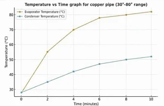
Fig. 3: Evaporator temperature (°C) and condenser temperature (°C) vs. time (minutes) for the copper heat pipe (30–80 °C range; averaged over three repeated trials, consistent with within the ±1 °C sensor resolution).
4.2 Conduction-based heat-transfer rate
This section is presented first because it is the analytically derived quantity that all subsequent phase-change and material-comparison calculations build on. The one-dimensional wall conduction model, applied to the measured evaporator–condenser temperature difference (ΔT = 50 K), gives a conservative lower-bound heat-transfer-rate estimate:
Q = kA(Te − Tc)/L
where A = (π/4)(D²outer − D²inner) = 6.597 × 10⁻⁵ m², ΔT = 50 K, and L = 0.204 m.
QCu = 400 × 6.597 × 10⁻⁵ × 50/0.204 ≈ 31.15 W
This 31.15 W figure is therefore analytically calculated from a measured temperature difference—it is not itself a directly measured heat-transfer rate. It is used below (Section 4.3) as a conservative lower-bound input to the phase-change estimate; no independent calorimetric measurement of heat input or heat transfer was obtained in this study (see Limitations, Section 5).
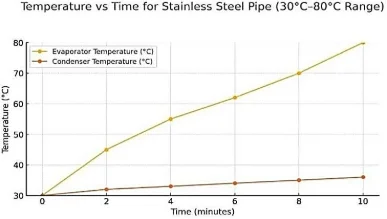
Fig. 4: Evaporator temperature (°C) and condenser temperature (°C) vs. time (minutes) for the stainless-steel case (30–80 °C range, simulated/analytical—not an independent SS304 experimental run; see Limitations).
4.3 Phase-Change heat transfer analysis
A heat pipe transfers heat primarily through the latent heat of vaporization, not through wall conduction alone. In this section, the phase-change contribution is characterized explicitly, using the conduction-based estimate from Section 4.2 as a conservative lower-bound input.
Qevap = ṁ × hfg
where ṁ is the vapor mass flow rate (kg/s) and hfg is the latent heat of vaporization of water at the operating temperature. At the measured evaporator steady-state temperature of ~80 °C:
hfg = 2308 kJ/kg[16]
Using the analytically derived, conservative lower-bound heat-transfer rate (Q = 31.15 W; Section 4.2) as input:
ṁ = Q/hfg = 31.15/(2308 × 10³) ≈ 1.35 × 10⁻⁵ kg/s
This represents a continuous cyclic flow of vapor from the evaporator to the condenser and the liquid condensate returning through the wick—the fundamental operating principle of the heat pipe. The effective thermal conductivity of the operating system over the vapor core cross-section is as follows:
Avapor = (π/4) × Dinner² = (π/4) × (0.0205)² = 3.30 × 10⁻⁴ m²
keff = Q × L/(Avapor × ΔT) = 31.15 × 0.204/(3.30 × 10⁻⁴ × 50) ≈ 385 W/m·K
This keff is defined over the vapor-core cross-sectional area (Avapor) and the axial evaporator–condenser ΔT as a means of expressing the phase-change transport on the same basis as a wall-conduction conductivity for comparison. It is strictly a derived lower-bound estimate rather than an independently measured effective thermal conductivity: it is built from the same conservative Q obtained from the measured ΔT (Section 4.2), not from an independent heat-flow measurement, and — as shown in Section 4.7 — is algebraically independent of ΔT itself under this model. In context, heat-pipe literature reports very high effective thermal transport capability relative to conventional solid conduction, and the present lower bound estimate (≥385 W/m·K) is well below that range; it should be read only as a floor consistent with phase-change transport being present, not as evidence quantifying its magnitude relative to wall conduction.[1,2] For stainless steel, a low wall conductivity (15 W/m·K) is estimated by the same scaling approach to prevent adequate heat flux delivery to the wick, which suppresses evaporation and results in a vapor flow rate approximately 27 times lower (ṁSS ≈ 5.07 × 10⁻⁷ kg/s), which is consistent with the high thermal resistance and steep temperature gradient reported for stainless steel casings in the literature; this SS304 figure has not been independently verified by experiments in the present study.[6,8]
4.4 Thermal resistance
Rth = ΔT/Q
Rth,Cu = 50/31.15 ≈ 1.605 K/W
This low value confirms excellent heat-spreading capability. The high thermal resistance of stainless steel (42.4 K/W, analytical) explains why its wall is predicted to be unable to sustain the phase-change cycle—sufficient heat would reach the working fluid at the evaporator to drive meaningful evaporation.[8]
4.5 Material comparison: copper vs stainless steel
Stainless steel 304 (k = 15 W/m·K) was compared with copper under identical conditions. SS304 was not independently manufactured or tested in this study; its performance was estimated by scaling the copper results by the ratio of wall thermal conductivities and rerunning the ANSYS model with the SS304 conductivity value. This is a simplified, single-parameter scaling: it holds geometry, wick, working fluid, and all boundary conditions fixed and varies only in terms of wall conductivity; thus, it does not capture any material-specific differences in wick wettability, capillary performance, or manufacturing tolerance that a real SS304 unit would exhibit (see Section 2, ref 6–8, and Limitations). Table 1 summarizes the full material comparison, including phase-change characterization, with each value explicitly labeled by its evidentiary basis.
QSS = QCu × (kSS/kCu) = 31.15 × (15/400) ≈ 1.17 W
Rth,SS = ΔT/QSS = 50/1.17 ≈ 42.4 K/W
Table 1: Comparison of the thermal performance of copper and stainless steel 304 under identical operating conditions. All copper values are derived from the single measured ΔT reported in Section 4.1; all the SS304 values are analytical/numerical estimates and have not been independently measured (see Limitations, Section 5).
| Property | Copper | Stainless Steel 304 | Observation |
|---|---|---|---|
| Thermal Conductivity | 400 W/m·K (manufacturer datasheet) | 15 W/m·K (literature value, assumed) | Copper ≈ 26.6× higher |
| Heat-Transfer Rate (Conduction) | 31.15 W — analytical, from measured ΔT | 1.17 W — analytical (scaled) | Copper ≈ 27× better |
| Thermal Resistance | 1.605 K/W — analytical | 42.4 K/W — analytical | Stainless steel highly inefficient |
| Vapor Mass Flow Rate | 1.35×10⁻⁵ kg/s — analytical (lower bound) | ~5.07×10⁻⁷ kg/s — analytical (scaled) | Copper sustains higher flow |
| Effective Thermal Conductivity | ≥385 W/m·K — analytical lower bound | — | Phase-change enhances copper |
| Temperature Gradient | Smooth (ANSYS, single-phase conduction model) | Sharp (ANSYS, single-phase conduction model) | Copper superior |
4.6 ANSYS temperature distribution and model validation
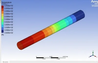
The ANSYS steady-state temperature contour for the copper heat pipe is shown in Fig. 5, and the corresponding simulation for stainless steel 304 is shown in Fig. 6. Correlating Figs. 5 and 6 with Table 1, the smooth, gradual color transition across the full pipe length in Fig. 5 corresponds to the low Rth of copper (1.605 K/W); the heat entering the evaporator is spread efficiently enough that the condenser end remains close to the evaporator temperature. In contrast, in Fig. 6, the temperature contour is concentrated almost entirely within the evaporator region, with the adiabatic and condenser sections remaining close to ambient—the visual counterpart of the high Rth of the SS304 (42.4 K/W; Table 1). Because both simulations use boundary conditions derived from the same underlying scaling relationship (Section 4.5), this graphical contrast and the tabulated Rth values are consistent with each other by construction rather than being two independent confirmations of the same physical claim.
4.6.1 Quantitative validation
The simulated steady-state copper ΔT (evaporator − condenser) was ≈43 K, against a measured ΔT of 50 K:
Percent error = |ΔTsim − ΔTexp|/ΔTexp × 100 = |43 − 50|/50 × 100 ≈ 14%
A 14% deviation between the single-phase conduction-only ANSYS model and the measured ΔT is a reasonable level of agreement given that the model excludes phase-change transport, radiation losses, and any parasitic conduction/convection losses along the adiabatic section insulation, but it is not close enough to describe the simulation as a precise match. We note explicitly that this is not a fully independent validation: the evaporator heat-flux boundary condition applied in the ANSYS model (Section 3.5.3) is itself analytically derived from the same measured ΔT that the simulation is then compared against, so some degree of agreement is expected by construction rather than demonstrated independently. A fully independent validation would require an evaporator heat input measured by a method separate from the temperature difference-based estimate (e.g., a metered LPG flow rate or an electrical heater of known power), which was not available in this study (see Limitations). The 14% figure is reported here as an explicit quantitative metric, superseding the qualitative "close agreement" wording used in an earlier version of this manuscript, but should be read with this caveat in mind.
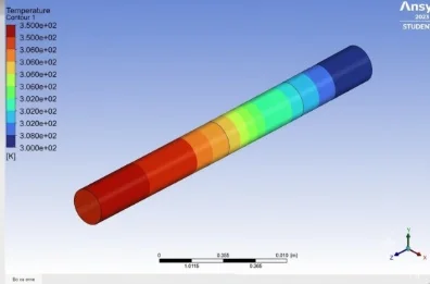
Fig. 5: ANSYS steady-state temperature contour for the copper heat pipe (single-phase, conduction-only solid-wall model). The smooth gradient from ~343 K (red, evaporator) to ~300 K (blue, condenser) is consistent with efficient axial heat spreading; the contour reflects the prescribed boundary conditions and does not resolve evaporation, condensation, or vapor transport (Section 3.5.1).
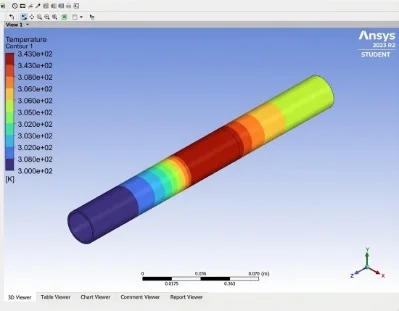
Fig. 6: ANSYS steady-state temperature contour for the stainless-steel case (single-phase, conduction-only solid-wall model, k = 15 W/m·K). The steep gradient and heat concentration at the evaporator are consistent with poor axial heat spreading under this scaling approach; as shown in Fig. 5, this is a thermal-field result under the prescribed boundary conditions, not direct evidence of suppressed phase-change activity.
4.7 Experimental uncertainty and repeatability
Each reported temperature is the average of three repeated trials under nominally identical conditions, recorded with a SOLARA Digital LCD Cooking Food Thermometer (stainless-steel probe, manufacturer-stated accuracy ±1 °C), and checked against an ice-water bath (0 °C reference) before testing. Readings were consistent across all three trials to within the ±1 °C instrument resolution, with no additional statistical scatter observed beyond this. Taking the sensor accuracy of ±1 °C on each of the evaporator and condenser readings, the propagated uncertainty on the evaporator–condenser temperature difference (ΔT = 50 K) is as follows:
δΔT = √[(δTe)² + (δTc)²] = √(1² + 1²) ≈ ±1.41 K
which corresponds to a relative uncertainty of ±1.41/50 ≈ ±2.8% on ΔT. Under the adopted conduction model, Q = kAΔT/L is directly proportional to ΔT; thus, this ±2.8% relative uncertainty propagates directly to Q: Q = 31.15 ± 0.87 W. Rth and keff, however, do not inherit this uncertainty in the same way. Algebraically, Rth = ΔT/Q = ΔT/(kAΔT/L) = L/(kA): the ΔT term cancels, so Rth depends only on the pipe geometry (A, L) and the material conductivity (k) and not on the measured temperature difference. Similarly, keff = QL/(AvaporΔT) = (kAΔT/L)·L/(AvaporΔT) = kA/Avapor, which also cancels ΔT entirely. The reported values (Rth = 1.605 K/W, keff ≥ 385 W/m·K) are therefore deterministic under this model given the assumed geometry and conductivity and are not subject to the ±2.8% ΔT-based uncertainty stated above for Q. Their actual uncertainty would instead come from geometric measurement tolerance (pipe diameters and length) and the manufacturer-stated conductivity value — neither of which was independently quantified with an error bound in this study — and we report this as a limitation rather than assign an unsupported error bar to Rth and keff. The LPG heat input was not independently met, so no formal uncertainty bound is placed on the source heat flux itself (see Limitations, Section 5).
5. Limitations
The following limitations bound the scope of the conclusions drawn in this study:
- The SS304 comparison is analytical/numerical only. No independent SS304 heat pipe was fabricated or tested; the reported 1.17 W, 42.4 K/W, and ~27× performance gaps follow from scaling the copper results by wall thermal conductivity, holding wick, working fluid, and geometry fixed. Real SS304 units may perform differently because of wick–fluid compatibility and manufacturing differences (Section 2, ref 6–8).
- The ANSYS model is a single-phase, conduction-only solid-wall representation. It does not resolve vapor–liquid two-phase flow, evaporation, condensation, or capillary wick transport; its temperature contours should be read as thermal-field validation under the prescribed boundary conditions, not as direct confirmation of phase-change phenomena.
- The ANSYS "validation" (Section 4.6.1) is not fully independent, since the evaporator heat-flux boundary condition is itself derived from the same measured ΔT that the simulation is compared against; a metered heat input (e.g., an electrical heater of known power) would be needed for a fully independent check.
- No mesh-independence study was performed for the ANSYS model (Section 3.5.2); the default program-controlled mesh was used throughout.
- The condenser heat-transfer coefficient (h = 25 W/m²·K) is an assumed representative value for low-velocity forced-air convection, not a measured quantity.
- The heat input of the LPG evaporator was not independently met, and heat loss along the adiabatic-section insulation was not separately quantified.
- Three temperature measurement locations (evaporator, mid-length adiabatic section, and condenser) were used; a finer axial resolution and any local hot/cold spots between these points were not resolved experimentally.
- Wick material and mesh specifications are now documented from the supplier's product listing (SS304 plain weave, 200 mesh, 0.050 mm wire diameter; Section 3.1) — a specification consistent with meshes typically used as capillary wicks in heat pipes. However, the supplier does not state porosity, permeability, or wick thickness, and the internal filling/sealing pressure was not recorded for this test article; these remain unquantified.
- Only three repeated trials were performed. Q has ±2.8% uncertainty in terms of sensor accuracy (Section 4.7); Rth and keff are deterministic under the adopted model given the assumed geometry and material conductivity, and their true uncertainty (from geometric tolerance and conductivity data) was not independently quantified.
6. Conclusion
In this study, how the pipe-wall material affects heat-pipe thermal performance was evaluated by combining direct experimental characterization of a copper–water heat pipe with an ANSYS single-phase thermal model and an analytical extension to stainless steel 304. With respect to the objectives stated in Section 1, the main conclusions, stated with their evidentiary basis, are as follows:
- The copper heat pipe achieved a measured steady-state ΔT of 50 K and — analytically derived from that measurement — a conduction-based Q = 31.15 W, thermal resistance = 1.605 K/W, and minimum vapor mass flow rate of 1.35 × 10⁻⁵ kg/s via the evaporation–condensation cycle. This directly addresses the study's first objective of characterizing copper–water performance under controlled laboratory conditions.
- Phase-change analysis indicates that the primary heat transport mechanism is evaporation–condensation (hfg = 2308 kJ/kg at 80 °C), yielding a lower bound effective conductivity ≥ 385 W/m·K, which is consistent with the high effective thermal conductivities reported for heat-pipe systems; this figure is a derived floor, not an independently measured effective conductivity (Section 4.3, 4.7).
- The single-phase ANSYS model reproduced the measured copper ΔT to within 14% (simulated ≈43 K vs. measured 50 K; Section 4.6.1), supporting the model as a reasonable thermal-field approximation under the stated assumptions; this comparison is not a fully independent validation, since the ANSYS boundary condition is itself derived from the same measured ΔT (see Limitations).
- Stainless steel 304 is analytically estimated to yield Q = 1.17 W and Rth = 42.4 K/W—under the wall-conductivity-only scaling approach used here, which is approximately 27 times worse than that of copper. ANSYS shows a correspondingly steep gradient under the same scaling; this SS304 result has not been independently validated by experiments and should be treated as a prediction, not a measured outcome. The literature on optimized stainless-steel wick designs indicates that this gap is a property of the present unmodified-wick scaling approach, not an intrinsic limit of stainless steel as a casing material (see Limitations).
- Within the tested configuration and the stated assumptions, copper outperforms the analytically scaled SS304 case for compact heat-pipe applications requiring fast, reliable thermal management; generalizing this to stainless-steel heat pipes with independently optimized wicks (ref. 6–10) requires further experimental validation.
Overall, the goal of this study is to quantify the impact of wall-material conductivity on heat-pipe performance within a transparent measured/analytical/simulated framework, whereas the limitations (Section 5) define the boundaries within which these conclusions should be read. Future work should incorporate full two-phase CFD modeling to explicitly resolve the vapor–liquid flow within the wick, conduct independent experimental testing of stainless-steel heat pipes with a wick optimized for that material rather than reusing the copper unit's wick design, meter the evaporator heat input independently of the temperature difference-based estimate to enable a fully independent ANSYS validation, perform a mesh-independence study for the ANSYS model, and investigate alternative wick structures, working fluids, and orientations.
Acknowledgment
The authors thank the Department of Mechanical & Automation Engineering, Pravin Rohidas Patil College of Engineering & Technology, Mumbai, for providing laboratory facilities and equipment for this study.
CRediT Author Contribution Statement
Karthik Tummalapalli: Conceptualization, Methodology, ANSYS simulation, Formal analysis, Writing – original draft, Writing – review & editing. Sahil Wagh: Experimental setup, Data collection, Investigation, Writing – review & editing. Hardik Dhumal: Data curation, Resources, Formal analysis, Writing – review & editing. Omkar Batwale: Validation, Visualization, Writing – review & editing. Vishal Kandalgaonkar: Supervision, Writing – review & editing. All the authors have read and approved the final version of the manuscript for publication and agree to be accountable for all aspects of the work, ensuring that questions related to the accuracy or integrity of any part of the work are appropriately investigated and resolved.
Funding Declaration
This research did not receive any specific grant from funding agencies in the public, commercial, or not-for-profit sectors.
Data Availability Statement
The experimental data and ANSYS simulation files supporting the findings of this study are available from the corresponding author upon reasonable request.
Conflict of Interest
There is no conflict of interest.
Artificial Intelligence (AI) Use Disclosure
The authors declare that artificial intelligence (AI)-assisted tools were used only for language refinement, grammar improvement, and manuscript structuring purposes during the preparation of this work. All technical content, experimental implementation, results, and interpretations were independently developed and verified by the authors.
Supporting Information
Not applicable.
References
- [1] A. Faghri, Review and advances in heat pipe science and technology, Journal of Heat Transfer, 2012, 134, 123001, doi: 10.1115/1.4007407.
- [2] L. L. Vasiliev, Heat pipes in modern heat exchangers, Applied Thermal Engineering, 2005, 25, 1–19, doi: 10.1016/j.applthermaleng.2003.12.004.
- [3] M. Mahdavi, S. Tiari, S. De Schampheleire, S. Qiu, Experimental study of the thermal characteristics of a heat pipe, Experimental Thermal and Fluid Science, 2018, 93, 292–304, doi: 10.1016/j.expthermflusci.2018.01.003.
- [4] R. Kempers, A. J. Robinson, D. Ewing, C. Y. Ching, Characterization of evaporator and condenser thermal resistances of a screen mesh wicked heat pipe, International Journal of Heat and Mass Transfer, 2008, 51, 6039–6046, doi: 10.1016/j.ijheatmasstransfer.2008.04.001.
- [5] N. S. D. Putra, W. N. Septiadi, H. Rahman, R. Irwansyah, Thermal performance of screen mesh wick heat pipes with nanofluids, Experimental Thermal and Fluid Science, 2012, 40, 10–17, doi: 10.1016/j.expthermflusci.2012.01.007.
- [6] X. Wang, Z. Wan, Heat transfer performance of a heat pipe with sintered stainless-steel fiber wick, Case Studies in Thermal Engineering, 2023, 45, 103016, doi: 10.1016/j.csite.2023.103016.
- [7] P. L. Reddy, B. S. Reddy, K. Govindarajulu, D. Bandhu, A. Saxena, Predicting the thermal performance of screen mesh wick heat pipe with alumina nanofluids using response surface methodology, International Journal on Interactive Design and Manufacturing, 2024, 18, 3167–3182, doi: 10.1007/s12008-023-01473-8.
- [8] E. F. de Araújo, J. P. Flórez Mera, L. H. R. Cisterna, M. B. H. Mantelli, New water-stainless steel rod-plate heat pipe: model and experiments, Heat and Mass Transfer, 2024, 60, 1073–1104, doi: 10.1007/s00231-024-03471-2.
- [9] J. Mansouri, I. Saad, S. Maalej, A. Driss, M. C. Zaghdoudi, Thermal performance evaluation of a water-filled axially grooved copper flat heat pipe for electronics cooling, Journal of Thermal Analysis and Calorimetry, 2022, 147, 8579–8612, doi: 10.1007/s10973-021-11099-1.
- [10] F. Xin, T. Ma, Q. Wang, Y. Yan, W. Tian, Thermal characterization and wick optimization of mini-grooved flat heat pipe for electronics cooling, Journal of Thermal Analysis and Calorimetry, 2022, 147, 14859–14872, doi: 10.1007/s10973-022-11739-0.
- [11] R. Scigliano, V. De Simone, R. Fusaro, D. Ferretto, N. Viola, Numerical Simulation of Heat Pipe Thermal Performance for Aerospace Cooling System Applications, Aerospace, 2024, 11, 85, doi: 10.3390/aerospace11010085.
- [12] I. Saad, S. Maalej, M. C. Zaghdoudi, Combined effects of heat input power and filling fluid charge on the thermal performance of an electrohydrodynamic axially grooved flat miniature heat pipe, Applied Thermal Engineering, 2018, 134, 469–483, doi: 10.1016/j.applthermaleng.2018.01.099.
- [13] S. C. Wong, M. S. Deng, Performance tests on triple composite mesh-groove-powder wicks in a visualizable flat-plate heat pipe, International Journal of Heat and Mass Transfer, 2024, 219, 124912, doi: 10.1016/j.ijheatmasstransfer.2023.124912.
- [14] W. Sanhan, R. Wanison, N. Kammuang-lue, P. Terdtoon, P. Sakulchangsatjatai, Experimental and numerical investigation of flattened and bent miniature heat pipes with two heat sources for laptop computers, Applied Thermal Engineering, 2023, 231, 120866, doi: 10.1016/j.applthermaleng.2023.120866.
- [15] A. B. Solomon, K. Ramachandran, L. G. Asirvatham, B. C. Pillai, Numerical analysis of a screen mesh wick heat pipe with Cu/water nanofluid, International Journal of Heat and Mass Transfer, 2014, 75, 523–533, doi: 10.1016/j.ijheatmasstransfer.2014.04.007.
- [16] W. Wagner, A. Pruß, The IAPWS Formulation 1995 for the Thermodynamic Properties of Ordinary Water Substance for General and Scientific Use, Journal of Physical and Chemical Reference Data, 2002, 31, 387–535, doi: 10.1063/1.1461829.
Publisher Note
Publisher Note: The views, statements, and data in all publications solely belong to the authors and contributors. GR Scholastic is not responsible for any injury resulting from the ideas, methods, or products mentioned. GR Scholastic remains neutral regarding jurisdictional claims in published maps and institutional affiliations.
Open Access
This article is licensed under a Creative Commons Attribution-NonCommercial 4.0 International License, which permits the non-commercial use, sharing, adaptation, distribution and reproduction in any medium or format, as long as appropriate credit to the original author(s) and the source is given by providing a link to the Creative Commons License and changes need to be indicated if there are any. The images or other third-party material in this article are included in the article's Creative Commons License, unless indicated otherwise in a credit line to the material. If material is not included in the article's Creative Commons License and your intended use is not permitted by statutory regulation or exceeds the permitted use, you will need to obtain permission directly from the copyright holder. To view a copy of this License, visit: https://creativecommons.org/licenses/by-nc/4.0/
© The Author(s) 2026