

 Open Access||Research Article
CNS-STGU Defense: Trust-Conditioned Cross-Dataset IoT Intrusion Detection with Unknown-Family Rejection and Drift-Aware Response Control
Atheer Alaa Hammad1 , Kavita S. Oza1, Kabir G. Kharade1
Department of Computer Science, Shivaji University, Vidya Nagar, Ujalaiwadi, Kolhapur, Maharashtra, 416004, India
Abstract
In the case of Internet of Things (IoT) intrusion detection, traffic classification is a necessary step, as well as a decision on whether there is enough evidence to warrant a response. This study introduces a trust-conditioned spatial–temporal framework, called CNS-STGU Defense, which splits these tasks. A typical representation is to map CICIoT2023 and TON_IoT Network to 6 behavioural families and 33 packet-derived descriptors, where the grouping of capture/device/session is done before fitted preprocessing and window construction. The encoder is defined by a one-dimensional convolutional neural network (CNN), bidirectional long short-term memory (BiLSTM) network and additive attention. Decision acceptance is based on calibrated probabilities, prototype distance, uncertainty and distribution monitoring, and simulator-ranked actions are limited by symbolic constraints. The provided 187,360-window reference matrix achieves 99.495% accuracy, macro-averaged F1 score (macro-F1) of 99.505%, Matthew’s correlation coefficient (MCC) of 0.9939 and false-alarm rate (FAR) of 0.603%. The macro-F1 for balanced transfer reconstruction is 94.207% and 94.707%. Evidence is broken down into matrix derived quantities (M), deterministic analytical calculations (A), and reconstructed or stated illustrations (R). The contribution consists of an auditable interface connecting prediction, acceptance and response constraints, numerical consistency analysis and a matched evaluation protocol. The illustrations of the transfer and gate do not constitute an empirical superiority. Retained predictions, fitting records and response logs are not provided here and must be validated.
Keywords
1. Introduction
The IoT networks are used to transport data from devices that have varying computing capabilities, update frequencies and service needs. Gateway level monitoring is a level where network observations can be used in intrusion detection and response.[1] A wrong automated action at this stage can disrupt the normal functioning of the services and the acceptance of a prediction is a different issue from the class label.[2]
Previous research has focused on deep architectures and feature reduction and graph-based representations of IoT traffic that incorporate local structure and temporal order. [3,4] The motivation for the representation used here comes from these studiesp.[5] Changes in capture environment, unsupported attack families and the limitations on potential responses should be taken into account when using classification scores for deployment evaluation.[6,7]
The first challenge comes when the assessment context changes. The traffic of the devices in an IoT network fluctuates depending on duty cycles, firmware and deployment conditions, and public benchmarks differ even more in terms of capture apparatus, feature schema and attack taxonomy. When repeated flows, source-specific artefacts and identity-bearing fields exist in the evaluation partition, high internal accuracy is not sufficient to establish transfer to another capture environment.
The second challenge is when a closed-set classifier is faced with traffic from outside the traffic families it knows: it still labels it with a known-family label. If the label is mapped directly to an action, the question of whether its probability is calibrated, its representation is supported, whether the traffic distribution is within scope, and whether the response is permissible remain unanswered. These questions stimulate a separate decision-acceptance stage. We use the framework name CNS-STGU Defense throughout this paper to refer to the trust-conditioned spatial–temporal intrusion detection with constrained response control. It provides separate prediction and trust and response interfaces to answer these four questions. The encoder provides a class prediction and behavioral context. The trust layer fuses together the probabilities of validation, entropy, class margin, prototype distance and drift state. The population stability index (PSI) is used to track the drift in the input-descriptors, and the Jensen–Shannon divergence (JSD) is used to track the joint predicted-family/confidence distribution. A simulator and symbolic rules then evaluate the actions of the candidates. This separation is not a proof of the effectiveness of the causal response, but an architectural contribution, and the change in the unit of evaluation that it suggests is stated in Fig. 1.
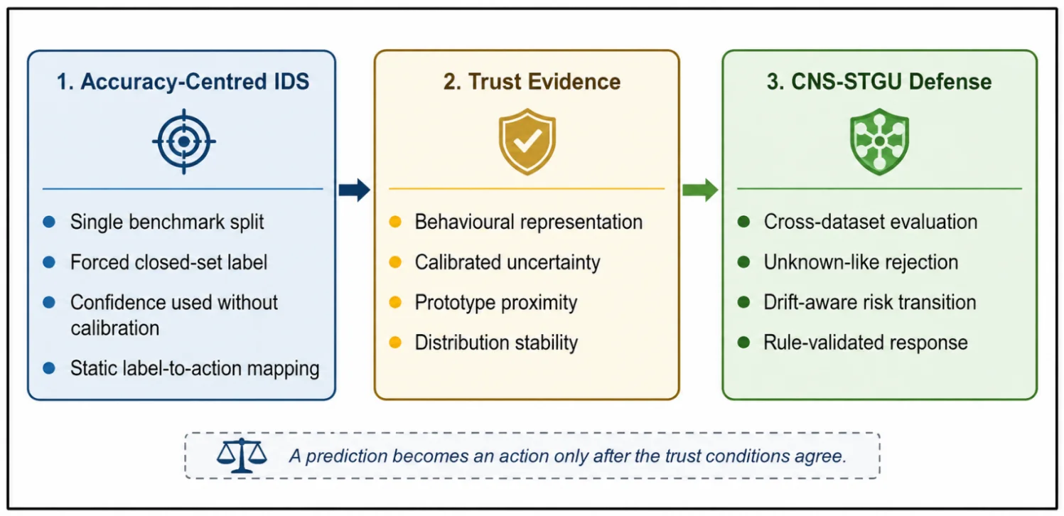
Fig. 1: Conceptual shift from score-centered classification to trust-conditioned decision support.
Fig. 1 distinguishes class prediction from decision acceptance. The encoder estimates a known-family label. The trust and policy stages determine whether the evidence supports a response. Unknown-like, shifted or ambiguous traffic can therefore be deferred without changing the underlying class prediction.
1.1 Research gaps
The research gap examined here is the absence of a demonstrated link, within the supplied evidence, between cross-source classification and the reliability of accepted responses. The proposed interface makes that link testable through four questions:
1. Does source-only evaluation remain valid when capture conditions, feature schemas and attack taxonomies differ?
2. Can unsupported families be deferred without an unacceptable rejection rate on known traffic?
3. Do calibration, prototype support and drift monitoring reduce error among accepted decisions at comparable coverage?
4. Do response constraints exclude inadmissible actions, and what additional review workload does this create?
1.2 Research objectives
The objectives specify the method and the comparisons needed to answer these questions. distinguishes the available numerical evidence using the convention.
I. Specify a common representation and group-isolated partition protocol for CICIoT2023 and TON_IoT, audit the supplied pooled count matrix, and define bidirectional source-only transfer.
II. Define a prediction-specific trust record containing calibrated confidence, entropy, class margin, prototype distance and drift state.
III. Specify matched rejection and gate comparisons, separating raw classification from accepted-decision error, coverage and review workload.
IV. Define and stress-test a symbolic response gate for accepting, deferring or rejecting candidate actions, without treating the simulator as evidence of live-network safety.
1.3 Contribution and testable scope
The contribution is a common decision record connecting three stages: a class prediction, the evidence for accepting it and the constraints on its response. The representation and group-isolated protocol specify what can be compared between sources. The reasons for the acceptance or deferral are observable in the trust record. The actions are then limited by symbolic rules, based on the risk-transition simulator. A response guard will override a favorable simulated utility. The testable claim is that these stages can enhance the quality of accepted decisions and the admissibility of responses without altering the raw class predictions. To establish that claim, matched comparisons must be made between the classifier and the trust gate stage and the constrained response stage, and error, coverage and review workload must be reported separately. Those comparisons are given. The present contribution does not set the interface and its numerical consistency but the empirical gain of the combined system. Unknown-like traffic is traffic that is rejected due to lack of evidence for a known-family decision. A holdout round where a family is intentionally not included in training, prototypes, calibration and threshold fitting. Such a benchmark holdout is smaller than finding a previously unknown vulnerability. The four illustrative rounds in this paper address the former question. we survey related work, we detail our method, and we describe our evaluation protocol, including the evidence-class convention. Results are presented with the evidence class indicated. The interpretation, reproducibility and limitations are discussed and the conclusion.
3. Proposed methodology
3.1 Problem definition and trust record
Let a window contain T ordered flow vectors, each with F = 33 harmonised descriptors:
Xi = [xi, 1, …, xi, T] ∈ ℝT × F, yi ∈ 𝒴, (1)
The target labels and the encoder-to-classifier mappings are defined below. The corresponding trust record follows.
Y = {Normal, DDoS, DoS, Malware, Recon, Web}, fθ(Xᵢ) = hᵢ, g(hᵢ) = zᵢ (2)
𝒯i = (ŷi, p̃i, Hi, Mi, Di, Δi), (3)
The quantities used to determine whether to accept or defer the trust record are stored in the trust record, along with the predicted family. It has a probability vector, which is scaled by temperature. Hᵢ is the normalised entropy, Mᵢ the top two margin, Dᵢ the nearest class-prototype distance and Δᵢ the drift state. The following are the definitions of the candidate actions. Predicted labels don't give permission for an automatic action.
A = {allow, monitor, review, block, isolate} (4)
3.2 Overall system architecture
Fig. 2 is a separation of representation learning and evidence assessment and response selection. The encoder provides logits and behavioral context. The trust stage evaluates support, uncertainty and shift, and the response stage uses operational constraints. The active decision boundary does not change directly when memory is admitted, but rather after the analyst approves the memory.
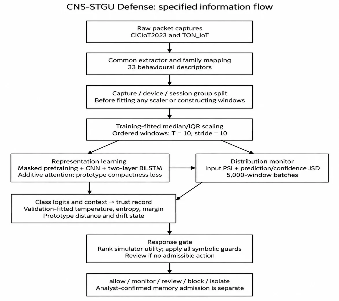
Fig. 2: Specified architecture with group isolation before fitted scaling and window construction.
Table 3 fixes the descriptor order. Packet definitions take precedence over processed-column aliases. The alias columns do not claim interchangeability with an existing CSV export. Raw captures, label associations and an executable extractor remain necessary for empirical reproduction. URI strings, certificate identities, addresses and capture metadata are excluded from model input.
3.3 Feature harmonization and leakage control
The manuscript introduces 46 CICIoT2023 and 43 TON_IoT Network fields that are used to start candidate
schemas. These counts are schema summaries and not the final input dimension.[17,18] The normative 33-descriptor specification is based on ordered packet records. Table 3 provides semantic aliases for orientation,
similarly named processed fields are not assumed to have the same units or aggregation. The packet-level
records are needed for particular statistics such as directional counts, packet inter-arrival statistics and TCP-
flag ratios. This specification requires source manifests and a versioned extractor to be used to link it to
benchmark windows. Ports, addresses, timestamps, dataset indicators and labels are not included in the model input, but can be used for service proxies and record or dering prior to removal.
ε = 10⁻⁸ (5)
Table 4 distinguishes operational metadata from model features. Timestamps and group identifiers are still needed for safe splitting and ordering, but are removed prior to scaling and training.
Table 3: Semantic aliases and the normative packet-based 33-descriptor specification
| No. | Unified descriptor | CICIoT2023 source or derivation | TON_IoT source or derivation |
|---|---|---|---|
| 1 | Flow duration | flow_duration / packet times | duration / connection times |
| 2 | Total packets | Number / packet count | src_pkts + dst_pkts |
| 3 | Forward packets | initiator-direction count | src_pkts |
| 4 | Backward packets | responder-direction count | dst_pkts |
| 5 | Total bytes | Tot size / byte sum | src_ip_bytes + dst_ip_bytes |
| 6 | Forward bytes | initiator-direction byte sum | src_ip_bytes |
| 7 | Backward bytes | responder-direction byte sum | dst_ip_bytes |
| 8 | Packets per second | Descriptor 2 / (duration + ε) | Descriptor 2 / (duration + ε) |
| 9 | Forward packets per second | Descriptor 3 / (duration + ε) | Descriptor 3 / (duration + ε) |
| 10 | Backward packets per second | Descriptor 4 / (duration + ε) | Descriptor 4 / (duration + ε) |
| 11 | Bytes per second | Descriptor 5 / (duration + ε) | Descriptor 5 / (duration + ε) |
| 12 | Mean packet size | Descriptor 5 / max(descriptor 2, 1) | Descriptor 5 / max(descriptor 2, 1) |
| 13 | Forward mean size | Descriptor 6 / max(descriptor 3, 1) | Descriptor 6 / max(descriptor 3, 1) |
| 14 | Backward mean size | Descriptor 7 / max(descriptor 4, 1) | Descriptor 7 / max(descriptor 4, 1) |
| 15 | Packet asymmetry | |Nf − Nb|/(N + ε), from ordered packets | same derivation |
| 16 | Byte asymmetry | |Bf − Bb|/(B + ε), from ordered packets | same derivation |
| 17 | Direction-change rate | Adjacent direction transitions / max(total packets − 1, 1) | Same derivation from ordered packets |
| 18 | Mean inter-arrival time | IAT mean / packet times | connection packet times |
| 19 | Inter-arrival SD | Std over IATs | SD over connection IATs |
| 20 | Minimum inter-arrival | minimum packet-time difference | same extraction |
| 21 | Maximum inter-arrival | maximum packet-time difference | same extraction |
| 22 | TCP indicator | TCP or Protocol Type | proto=tcp |
| 23 | UDP indicator | UDP or Protocol Type | proto=udp |
| 24 | ICMP indicator | ICMP or Protocol Type | proto=icmp |
| 25 | SYN ratio | TCP SYN count / (total packets + ε) | TCP SYN count / (total packets + ε) |
| 26 | ACK ratio | TCP ACK count / (total packets + ε) | TCP ACK count / (total packets + ε) |
| 27 | RST ratio | TCP RST count / (total packets + ε) | TCP RST count / (total packets + ε) |
| 28 | FIN ratio | TCP FIN count / (total packets + ε) | TCP FIN count / (total packets + ε) |
| 29 | HTTP indicator | Port 80 proxy; alias HTTP is contextual only | Same port 80 proxy; processed service alias is contextual only |
| 30 | HTTPS indicator | Port 443 proxy; alias HTTPS is contextual only | Same port 443 proxy; processed service alias is contextual only |
| 31 | DNS indicator | Port 53 proxy; alias DNS is contextual only | Same port 53 proxy; processed service alias is contextual only |
| 32 | SSH indicator | Port 22 proxy; alias SSH is contextual only | Same port 22 proxy; processed service alias is contextual only |
| 33 | Other-service indicator | Neither endpoint supplies a recognised service port | Same deterministic service fallback |
Table 4: Leakage-prone fields and their treatment
| Field group | Examples | Treatment | Reason |
|---|---|---|---|
| Identity | source/destination IP, MAC, flow ID | Removed | Device or capture memorisation |
| Endpoint | raw source/destination ports | Removed; service retained | Port can encode scenario construction |
| Time | timestamp, date, capture order ID | Used for grouping/order, then removed | Prevent direct temporal leakage |
| Dataset provenance | file, scenario, source dataset | Split control only | Prevent source classification |
| Target proxies | label, type, attack name | Target construction only | Direct label leakage |
| Sparse content | URI, user agent, certificate subject | Removed | Non-shared high-cardinality artefacts |
3.3.1 Deterministic common-extractor procedure
The reference procedure is a packet-by-packet processing of packets in each bidirectional flow. The first observed endpoint is the one that is the initiator. Let N and B be the number of packets and bytes respectively, and Nf, Nb, Bf and Bb be the number of packets and bytes in the forward and backward directions respectively. The following definitions are used for duration, rates and mean sizes.
d = tₙ − t₁ (6)
$R_{N} = rac{N}{d + arepsilon} R_{B} = rac{B}{d + arepsilon} S = rac{B}{max(N, 1)}$ (7)
The same definitions apply to directional counts. Packet and byte asymmetry use absolute directional differences. Let Kdir be the number of transitions between adjacent packet directions and Nflag the number of packets carrying a specified TCP flag. The protected ratios are
$Packet asymmetry = rac{|N_{f} - N_{b}|}{N_{f} + N_{b} + arepsilon} Byteasymmetry = rac{|B_{f} - B_{b}|}{B_{f} + B_{b} + arepsilon}$ (8)
$Direction - change rate = rac{K_{dir}}{max(N - 1, 1)} Flag ratio = rac{N_{flag}}{N + arepsilon}$ (9)
Table 3 is always used for the protective constant. The inter-arrival sequence is determined by the differences in the timestamps. It is characterized by its mean, population standard deviation, minimum and maximum form descriptors 18-21. Descriptors 22-33 are for protocol and service indicators. Changes the timeout, byte-counting, service and singleton conventions to be the reference specification; the only way to know if a historical extraction was performed with these settings is to have aggregate counts. The extraction sequence is: Packet ordering, Direction assignment, Count and duration calculation, Rate and ratio calculation, Inter-arrival statistics, Protocol/service encoding, Concatenation in the Table 3 order. Medians and interquartile ranges (IQR) are then used to assign the partitions. No scaling parameter is fitted on the validation or test records.
3.3.2 Reference extraction conventions
There are the following options that define one consistent reference extraction and windowing protocol. They are not settings to verify the completion of a raw-capture run. The reference extractor works on packets in a bidirectional 5-tuple in a chronological manner. If the gap between the previous packet is more than 30 s, or the time from the first packet is more than 120 s, a new flow will start. The first observed endpoint is the one that is the initiator. The input order is preserved for equal packet timestamps. The byte count is for complete IP packets, and does not include link-layer headers. Upstream is a place where a fragment reassembly is needed. The relationship between packet-level attack labels and flow labels should be specified in the capture manifest.
If the flow is a singleton, all the duration and inter-arrival statistics are zero. Protected rates are finite but can be high, and are clipped by training quantiles prior to scaling by each descriptor. Service flags are not application inspection, but rather proxies of the service. The responder port is checked first, if it is not one of 80, 443, 53 or 22, then the initiator port is checked, otherwise the other-service flag is set. The five service indicators are mutually exclusive. Both sources are subject to the packet-based definitions. The reference interface is a packet record with timestamps, protocol, endpoints, byte counts and TCP flags. Timestamps and/or byte counts are not valid. The non-TCP flag ratios are all zero. Grouping is supported by identity fields and they are excluded from the model input. This manuscript does not include an executable package or its version identifier. Groups are determined prior to fitted clipping, scaling and windowing. Clipping is done with training quantiles of 0.001 and 0.999. Scaling is done using training medians and IQRs with a minimum of 10⁻⁸. The flow records in each window are 10 consecutive flow records, no window overlaps with another window, and the flow records in each window cannot cross a group boundary; the flow records in the remainder are dropped. A window is Normal if all the records are Normal. Otherwise, it is the most common malicious family (excluding Normal records for that vote), and the new malicious record in tied families is a tie-breaker. This is the same rule. Table 5 summarizes the fixed descriptor ordering and packet-based extraction conventions used to construct the 33-dimensional common representation across the two data sources.
Table 5: Descriptor order and packet-based reference conventions
| IDs | Descriptors | Definition |
|---|---|---|
| 1–4 | Duration, total/forward/backward packets | d = last time − first time, N, Nf, Nb |
| 5–7 | Total/forward/backward bytes | B, Bf, Bb |
| 8–11 | Total/forward/backward packet rate, byte rate | N/(d+ε), Nf/(d+ε), Nb/(d+ε), B/(d+ε) |
| 12–14 | Total/forward/backward mean packet size | B/max(N,1), Bf/max(Nf,1), Bb/max(Nb,1) |
| 15–17 | Packet/byte asymmetry, direction changes | |Nf−Nb|/(N+ε), |Bf−Bb|/(B+ε), K/max(N−1,1) |
| 18–21 | IAT mean, population SD, minimum, maximum | Consecutive timestamp differences, ddof = 0 |
| 22–24 | TCP, UDP, ICMP indicators | Three protocol flags |
| 25–28 | SYN, ACK, RST, FIN ratios | Flag packet count/(N+ε) |
| 29–33 | HTTP, HTTPS, DNS, SSH, other service | Responder port, then initiator: 80/443/53/22; otherwise, other |
3.4 Label harmonization
These are umbrella behavioral families of six labels for this evaluation. The scope retained in Table 6 is not a statement of equivalence of source attack mechanisms, but rather a definition of the scope. Brute Force/Spoofing and password/mitm are not included in the evaluated taxonomy. Their absence does not indicate that no cross-source counterpart could be defined, it is a scope choice.
Table 6: Source-to-unified label map
| Unified family | CICIoT2023 labels | TON_IoT labels | Decision |
|---|---|---|---|
| Normal | Benign | normal | Include |
| DDoS | DDoS category | ddos | Include |
| DoS | DoS category | dos | Include |
| Malware | Mirai category | backdoor, ransomware | Merge at malware-behaviour umbrella level |
| Recon | Recon category | scanning | Include |
| Web | Web-based category | injection, xss | Include |
| Excluded | Brute Force, Spoofing | mitm, password | Outside evaluated taxonomy; no mapped pair tested |
Umbrella behavioural families are defined in Table 6. The Malware family combines Mirai with backdoor/ransomware for this evaluation only, and does not claim equivalence of mechanisms nor provide fine-grained attribution. This is a general mapping that restricts the interpretation of transfer performance.
3.5 Grouped split and sequence construction
Capture/device/session groups must be in a single partition. Group identities must be provided with a source manifest and must be grouped with other sessions that would otherwise result in leakage. Flow records are sorted by start time, and then by a deterministic canonical flow-key tie-break. The T = 10 records in windows are not allowed to span groups and partitions. If all records are Normal, then the window is Normal. If not, the label is provided by the other malicious family, and in the case of tied families, the latest malicious record determines the label. For instance, a DDoS window is made up of nine Normal records and one DDoS record. The training-only clipping and median/IQR scaling are given. The length T of the windows records flow, not seconds. The period of time represented is defined below. Its distribution is reported in Fig. 12 for a time window of ten records. Window formation and model inference are two different latency components: a streaming decision also relies on the timing of the records that are needed.
Δtwindow = t10 − t1 (10)
Table 7 shows a total of 1,122,475 windows from the source and partition. They are not "capture counts" that have been reconstructed independently, but rather the declared ledger. The intended proportion is 2/3:1/6:1/6, small numerical deviations are acceptable for group allocation, but not for determining the cause of the deviation without group manifests. The number of tests (187,360) is the same as the denominator of the provided pooled reference matrix. That equality is not an equality of groups, but an equality of numbers.
Table 7: Declared pooled window-count ledger; provenance requires split manifests
| Source | Training | Validation | Test | Total |
|---|---|---|---|---|
| CICIoT2023[30] | 438,286 | 109,568 | 109,668 | 657,522 |
| TON_IoT Network[31] | 309,977 | 77,284 | 77,692 | 464,953 |
| Total | 748,263 | 186,852 | 187,360 | 1,122,475 |
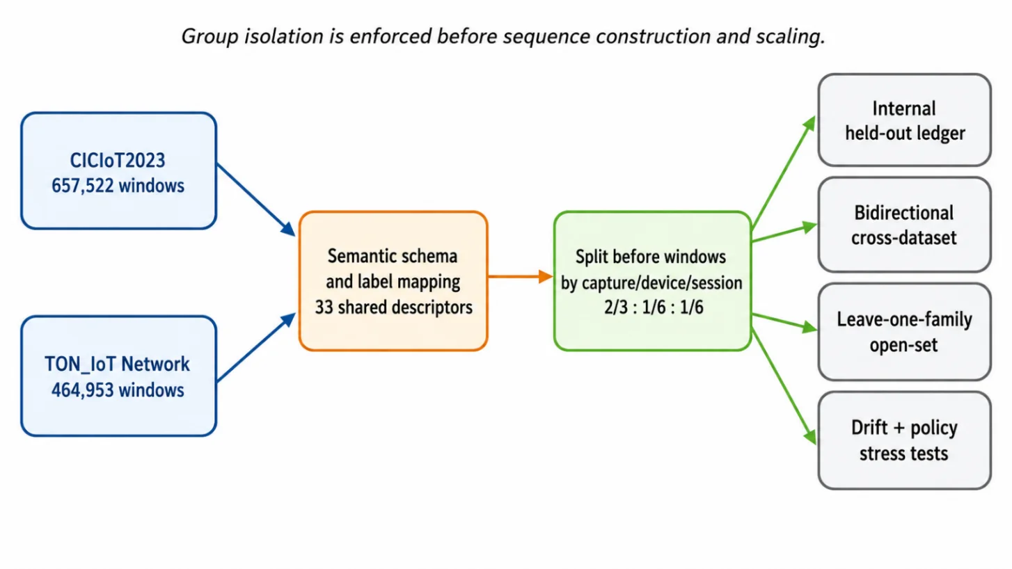
Fig. 3: Leakage-controlled evaluation protocol
The separation of internal, transfer, holdout and stress-test questions is planned as shown in Fig. 3. The totals in the dataset are for constructed windows, not pre-split packets. Fitted scaling and sequence construction must be done after group isolation. Test streams are not allowed to select the following settings: validation-only fitting, temperature, prototype-distance transforms and rejection thresholds.
Family totals are shown in illustrative form in thousands in Fig. 4. Its source sums are 657,000 and 465,000, compared with the declared exact totals 657,522 and 464,953 in Table 7. These approximations are not to be used as class support denominators. The reference matrix and Table 15 provide pooled test supports for exact tests; source-specific family manifests are not available.
3.6 Spatial-Temporal Representation Learning
The proposed pretraining stage is based on training partitions only. A Bernoulli mask is used to select 15% of the time-feature positions and the reconstruction loss is averaged over the selected positions. If the mask is
empty, it will not add any loss. No validation, test or held-out-family record is used during representation pretraining:
$mathcal{L}_{mask} = rac{1}{left| mathcal{M} ight|}sum_{(t,j)mathcal{in M}}^{}{Huber}left( x_{t,j},{widehat{x}}_{t,j} ight).$ (11)
The proposed supervised encoder consists of two 1D convolutional blocks, each having 64 and 128 filters and kernel size 3. The complete block Bℓ consists of a biased convolution, batch normalization, GELU and dropout 0.20. It is output in the following sequence:
St = [B₂(B₁(X))]t (12)
A two-layer BiLSTM with 128 units per direction produces gt = [g⃗t; g⃖t]. Additive attention computes
$e_{t} = v_{a}^{ op} anhleft( W_{a}g_{t} + b_{a} ight),quadalpha_{t} = rac{expleft( e_{t} ight)}{sum_{k = 1}^{T}expleft( e_{k} ight)},quad h = sum_{t = 1}^{T}alpha_{t}g_{t}.$ (13)
The classifier probability is p = softmax(Wch + bc). Class prototypes are exponentially updated training-set centroids,
$mu_{c} leftarrow homu_{c} + (1 - ho) rac{1}{left| B_{c} ight|}sum_{i in B_{c}}^{}h_{i},quadquad ho = 0.99,$ (14)
The prototype compactness penalty uses the sum of squared differences across all 256 context coordinates, averaged over the batch. It is not divided by 256:
$mathcal{L}_{proto} = rac{1}{|B|}sum_{i in B}^{} parallel h_{i} - mu_{y_{i}} parallel_{2}^{2}.$ (15)
The supervised data objective retains the masked reconstruction term as an auxiliary loss:
ℒ=ℒCE + 0.05ℒproto + 0.10ℒmask, (16)
In Eq. (16), the cross-entropy is weighted by the inverse of the training supports. The displayed data objective is added to the L2 weight penalty shown in Table 13, to provide the full optimization objective. Masked reconstruction is performed during supervised training (at weight 0.10) with a decoder that is attached to the training representation, but not used for inference. Prototype compactness is the average of the squared Euclidean distances over windows (not normalized by coordinates). Prototype dispersion and later rejection score are fitted separately and are not considered to be independent uncertainty signals.
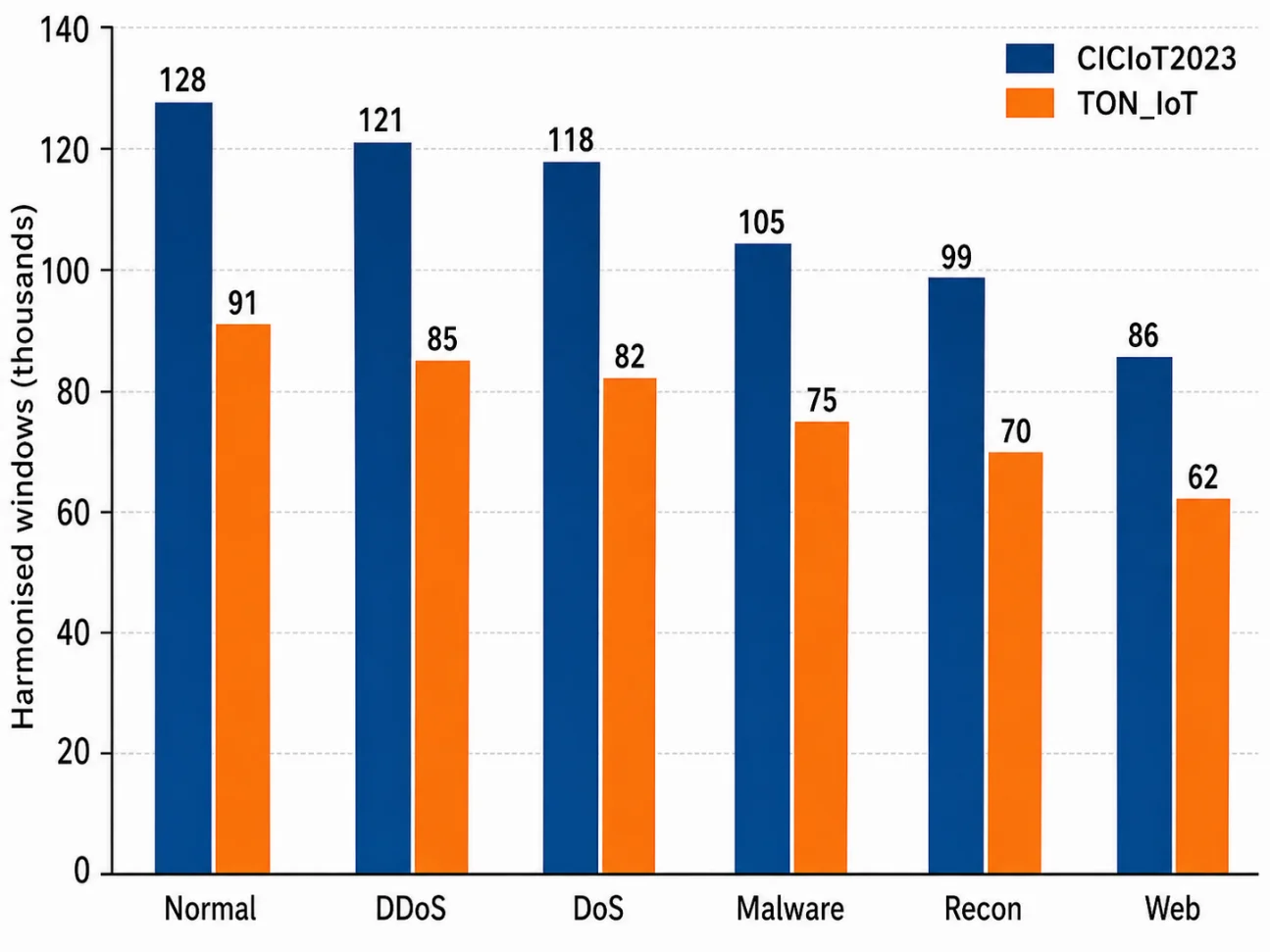
Fig. 4: Stated approximate family distribution by source (Class R).
3.7 Calibration, unknown-like rejection, and drift monitoring
Temperature τ > 0 is fitted by minimising validation negative log-likelihood (NLL) and is frozen for testing:
${widetilde{p}}_{c} = rac{expleft( z_{c}/ au ight)}{sum_{k}^{}expleft( z_{k}/ au ight)}.$ (17)
Normalized entropy and margin are
$H = - rac{1}{log C}sum_{c = 1}^{C}{widetilde{p}}_{c}logleft( {widetilde{p}}_{c} + epsilon ight),quadquad M = {widetilde{p}}_{(1)} - {widetilde{p}}_{(2)}.$ (18)
Prototype distance is normalized by validation dispersion sc:
$D = min_{c} rac{| h - mu_{c}| ₂}{max(s_{c}, arepsilon)}$ (19)
The rejection score combines complementary prototype-distance, entropy and margin signals:
U = 0.45D* + 0.35H + 0.20(1 − M), (20)
s_c is the root mean squared Euclidean distance between the correctly classified known validation contexts and the training prototype for each class, where ε is the floor. If there is no eligible validation context, then the class is invalidated and the round of the calibration is reported. The empirical validation cumulative distribution function (CDF) of D is the percentile rank of D. The rejection threshold is the 98.65th percentile of scores for correctly classified known validation windows (interpolated between ordered scores). Known-test false rejection: All known test windows are used. Each holdout has its own prototypes, dispersions, distance CDF and threshold, and is not included in any of the fittings.
For a monitored descriptor with reference-bin proportions qb and current proportions rb,
$PSI = sum_{b}^{}left( r_{b} - q_{b} ight)log rac{r_{b} + epsilon}{q_{b} + epsilon}.$ (21)
For the reference and current distributions, P and Q denote histograms over a fixed joint partition of predicted family and maximum-confidence bin. JSD uses natural logarithms and the same bins in both streams:
$JSD(P,Q) = rac{1}{2}KL(P parallel M) + rac{1}{2}KL(Q parallel M),quad M = rac{1}{2}(P + Q).$ (22)
A monitoring batch is assigned to shifted, warning or stable status by the numbered rule below. The precedence makes the categories mutually exclusive. The thresholds are specified operating conventions; the supplied stress scenarios do not establish their universal validity.
shifted ⇔ max(PSI) ≥ 0.25 ∨ JSD ≥ 0.05 (23)
warning ⇔ ¬shifted ∧ [max(PSI) ≥ 0.10 ∨ JSD ≥ 0.03] (24)
stable ⇔ max(PSI) < 0.10 ∧ JSD < 0.03 (25)
3.8 Structural risk-transition simulator and symbolic policy
The action layer is a bounded numerical simulator. Its state is x = (r, u, d, s), where r is assigned base risk, u is assigned uncertainty, d is assigned drift intensity and s is assigned service importance, each in [0,1]. These scenario inputs are not calibrated probabilities. The continuous d is distinct from the categorical stable/warning/shifted status used by routing rules. The one-step transition has a single form:
rnext(a) = clip[r(1 − ea) + αuu + αdd, 0, 1] (26)
Here e_a is the assigned action effect, α_u = 0.05 and α_d = 0.03. Disruption cost c_a enters the utility rather than the transition. The simulator is conditional on these inputs; it is not an estimate of causal intervention effects on a live network.
The candidate utility is
J(a | x) = rnext(a) + λccas, λc = 0.60 (27)
and the selected action is
a* = arg mina ∈ A : R(x, a) = 1 J(a | x) (28)
Minimizing J over the admissible set is equivalent to ranking. Lower disruption cost is the deciding factor for exact objective ties. When several routing rules apply, their allowed network-action sets are intersected, and disruption guards take precedence. If no network action is admissible, the system does not claim a network-risk-reduction, but defers to analyst review. Separate memory admission. Table 10 sets the admissible sets for the numerical scenarios, while the input predicates not listed in the table are assumed to be scenario conditions
Table 8 lists the routing that is allowed for the given predicates. Ambiguity and critical-service constraints are not subject to override by a lower simulated risk. The rule set is used to establish an admissibility boundary, and the impact of the rule set on operational outcomes must be assessed separately.
3.8.1 Numerical instantiation of the reference policy
The numerical instance uses base risks 0.12, 0.93, 0.88, 0.56 and 0.81. These are given scenario inputs. The same transition and utility as Eqs. is evaluated. The following are the coefficients of the equations (26–27). There is no second policy model used. The state notation is the same. The equations below replace the constant coefficients with the actual ones in the general transition and utility. The chosen action is the one that minimizes the objective in the scenario admissible set, and is the one that minimizes the disruption cost in case of a tie.
x = (r, u, d, s) (29)
rnext(a) = clip[r(1 − ea) + 0.05u + 0.03d, 0, 1] (30)
J(a) = rnext(a) + 0.60 ca s (31)
Table 8: Explicit symbolic response rules
| Rule | Predicate | Allowed outcome | Disallowed outcome |
|---|---|---|---|
| Rule 1 Stable benign | Normal, H < 0.25, D* < 0.60, stable | allow / monitor / review | isolate normal traffic |
| Rule 2 High-confidence flood | DDoS/DoS, M > 0.70, stable/warning | monitor / review / block, subject to guards | allow high-risk flood |
| Rule 3 Malware containment | Malware, maximum probability > 0.95, stable or warning; containment guards pass | isolate if guards pass; otherwise defer to review | allow or passive monitor |
| Rule 4 Boundary caution | Normal/Recon top-two pair and M < 0.25 | review/monitor | automatic block |
| Rule 5 Unknown under shift | U > γ and shifted | review; isolate only if every disruption guard passes | allow |
| Rule 6 Critical-service guard | Service importance s > 0.8 and evidence not unanimous | review before disruption | automatic isolate |
| Rule 7 Memory admission | analyst-confirmed, deduplicated, drift-tagged | Memory admission after review; not a network action | self-labelled insertion |
Table 9: Assigned simulator action effects and disruption costs
| Action | Effect e | Cost c |
|---|---|---|
| Allow | 0.00 | 0.00 |
| Monitor | 0.15 | 0.03 |
| Review | 0.30 | 0.06 |
| Block | 0.75 | 0.12 |
| Isolate | 0.85 | 0.25 |
Table 10: Assigned scenario states and fixed admissible action sets
| State | r | u | d | s | Admissible actions |
|---|---|---|---|---|---|
| Stable Normal | 0.12 | 0.05 | 0.03 | 1.00 | Allow, monitor, review |
| DDoS | 0.93 | 0.10 | 0.12 | 0.20 | Monitor, review, block |
| Malware | 0.88 | 0.08 | 0.08 | 0.30 | Isolate |
| Recon boundary | 0.56 | 0.55 | 0.18 | 0.80 | Monitor, review |
| Unknown + drift | 0.81 | 0.82 | 0.46 | 0.70 | Review |
Allow, monitor and review are permitted under the stable-Normal scenario. The DDoS scenario allows monitor, review and block. Isolate is allowed in the Malware containment scenario, but not in the Monitor scenario, per Rule 3. Monitor and review is allowed for the Recon boundary. If the unknown-plus-shift scenario is assumed, then it is specified that containment guards will fail, and only review will be assumed. All five candidate risks can be computed for each state, but only the fixed admissible set is used for selection. The effect assigned to review is an assumed completed analyst mediated response on the next horizon. Just adding an item to a review queue does not have an immediate network effect. All action effects and costs are assumed in the simulator. Numerical consequences are not measured outcomes of intervention.
3.9 Controlled continual memory
The proposed memory buffer stores up to 2,000 windows, evenly distributed among family and drift strata, that have been confirmed by analysts. It is designed with 20% stable-reference reservoir and cosine-similarity deduplication. One of the possible parameter regularization mechanisms is elastic weight consolidation:[16]
$mathcal{L}_{adapt} = mathcal{L}_{CE} + rac{lambda}{2}sum_{j}^{}F_{j}left( heta_{j} - heta_{j}^{old} ight)^{2}.$ (32)
No experiment of longitudinal adaptation is reported here. Thus, controlled memory is not a demonstrated reduction in catastrophic forgetting, but rather an implementation design that is bounded and a future evaluation target.
4. Experimental setup and evaluation protocol
4.1 Research questions and fixed protocol
The evaluation distinguishes between reference-matrix arithmetic, deterministic analytical calculations and illustrative scenarios, in the evidence convention. The proposed evaluation protocol is determined by the configuration choices, not by an archived training or device run. The separate records are required for source-only transfer, rejection and acceptance. There are 46 and 43 fields in the declared candidate schemas before harmonization to 33 descriptors based on the packets. Table 7 assigns 657,522 and 464,953 windows to the two sources, for 1,122,475 in total, with 748,263 training, 186,852 validation and 187,360 test windows. These are window counts and not packet counts. The only test data that can be recovered directly from the provided reference matrix is the pooled test support. The specification and numerical summaries are organized by 5 evaluation questions.
Internal discrimination: What class-count performance is implied by the pooled held-out reference matrix?
Cross-dataset transfer: How should a model trained on one source be evaluated on the other using the same feature and label mapping?
Unknown-family rejection: Can an attack family excluded from every fitting stage be identified as unsupported at test time?
Calibration and distribution shift: How should validation-fitted confidence and changes in the monitored traffic distribution be assessed separately?
Constrained response selection: Which actions remain permissible after symbolic rules are applied to simulator-ranked candidates? Report the permitted action, decision coverage and error among accepted decisions.
Table 11: Reference training and profiling configuration
| Item | Fixed value |
|---|---|
| Input | 10 × 33, non-overlapping grouped windows |
| CNN | 64/128 filters; kernel 3; batch norm; GELU; dropout 0.20 |
| BiLSTM | 2 layers; 128 units per direction |
| Attention/context | additive attention; 256-dimensional context |
| Optimiser | Adam; learning rate 10⁻³; L2 coefficient 10⁻⁵ (Table 13) |
| Batch and epochs | 64; maximum 12 epochs; best checkpoint by validation accuracy; patience 3 |
| Pretraining | 15% mask; 8 epochs; Huber reconstruction loss |
| Class control | inverse-frequency training weights; no test resampling |
| Seed labels for illustrative series | 11, 23, 37, 51, 71 |
| Software | Target stack: Python 3.10, TensorFlow/Keras, scikit-learn, NumPy, Pandas; exact builds unavailable |
| Hardware | Reference profile assumption: Tesla T4, Intel Xeon CPU, 16 GB RAM; run logs unavailable |
The intended encoder configuration is Adam with learning rate 10⁻³, L2 penalty coefficient 10⁻⁵ (Table 13), batch size 64 and at most 12 supervised epochs with patience 3 (Table 11). Validation accuracy is used for checkpoint selection and macro-F1 is the main reporting metric. The objective of Eq. (16) is used in the supervised training phase, with 8 epochs of pretraining using 15% masking. These settings are not a checkpoint that has been archived, nor are they a completed training run.
4.1.1 Evaluation populations and model configuration
Table 12 distinguishes the supplied aggregate matrix from illustrative per-window populations. Expanding a count matrix into labelled rows does not recover the original sample identities, captures, logits or predictions.
A is CICIoT2023 and B is TON_IoT throughout. It is assumed that there are 10,000 windows per family for each Class R transfer target, not the natural distribution of targets. The five primary seed labels are 11, 23, 37, 51 and 71; the extended stated series adds 89, 103, 127, 149 and 173. The assigned calibration-validation size 46,840 is 25.068% of the stated 186,852-window validation pool, which is 127 windows larger than an exact quarter. These arithmetic relationships do not form a group stratified extraction. How calibration subset is
selected from validation groups must be documented in executed evaluation.
Table 12: Reference and illustrative evaluation populations with provenance
| Population | Records | Interpretation |
|---|---|---|
| Illustrative per-window reference expansion | 187,360 | Assigned rows expanded from the supplied six-class matrix; original identities/logits not recovered |
| Assigned calibration-validation population | 46,840 | Illustrative size, 25.068% of stated validation pool; group membership unavailable |
| Illustrative A→B target | 60,000 | Assumed 10,000 windows per family |
| Illustrative B→A target | 60,000 | Assumed 10,000 windows per family |
| Open-set, each of 4 rounds | 5,000 / 10,000 / 2,500 | Known validation / known test / unknown test |
Table 13: Reference model configuration and optimization convention
| Setting | Assigned value |
|---|---|
| Input and window stride | 10 × 33 descriptors, stride 10 records |
| CNN blocks | 64 then 128 filters, kernel 3, stride 1, same padding, biases enabled |
| Normalisation and activation | BatchNorm ε = 0.001, momentum = 0.99, GELU |
| CNN dropout | 0.20 after each block |
| BiLSTM | 2 layers, 128 units per direction, sequences retained, recurrent dropout 0 |
| Additive attention | 256-dimensional hidden projection, trainable projection bias and score vector |
| Classification head | Dense 6 with bias, followed by softmax |
| Optimiser | Adam, initial learning rate 0.001, β₁ = 0.9, β₂ = 0.999, ε = 10⁻⁷ |
| Weight penalty | 0.5 × 10⁻⁵ × ||W||² added to loss, excluding biases and BatchNorm |
| Schedule and clipping | Constant learning rate, gradient global norm clipped to 1.0 |
| Batch and supervised epochs | Batch 64, maximum 12 epochs, patience 3, min_delta 0 |
| Checkpoint selection | Highest validation accuracy, earliest checkpoint breaks exact ties |
| Pretraining | 8 epochs, 15% independent position masking, Huber δ = 1 |
| Supervised objective | Weighted cross-entropy + 0.05 prototype compactness + 0.10 masked loss; add the stated L2 penalty |
| Prototype penalty | Squared Euclidean context-to-prototype norm, averaged over windows; no division by 256 |
| Initialisation | Glorot input weights, orthogonal recurrent weights, forget-gate bias 1 |
| Seeds | Primary robustness: 11, 23, 37, 51, 71; extended paired analysis additionally: 89, 103, 127, 149, 173 |
| Temperature fitting | Validation NLL minimisation over τ ∈ [0.25, 4.00] |
| Calibration summaries | 15 equal-frequency confidence bins, multiclass Brier summed across 6 classes |
The inference parameter calculation is the encoder and classification head in Table 13, without the residual branch, pooling layer before the recurrent stack or recurrent projection. The context-weighted sum of attention is added to the attention. The training-only reconstruction decoder is not included in the inference parameters and operations, and the layer configuration should be provided for reproducible training.
4.2 Baselines, transfer, and open-set tests
The proposed classification comparison comprises a deep neural network (DNN), CNN, long short-term memory (LSTM), BiLSTM and CNN–BiLSTM models. The pooled run would be using both training sources, and the source-only internal runs would train separate models. Transfer must be source only training, scaling and calibration, with no fine tuning, and then target testing. The holdout protocol is for Web, Recon, Malware and DoS, each in turn. Known: Normal and DDoS. No held-out-family example can be used in pretraining, supervised fitting, prototype estimation, calibration and threshold selection. The rejection comparison is based on maximum SoftMax probability, energy scoring, Mahalanobis distance, OpenMax and prototype-only scoring and prototype plus uncertainty.[20,21,22,23] The comparison is conducted over the same four-family scope and the same known-traffic false-rejection denominator, thus enabling the score definitions and thresholds to be directly compared. This comparison is instantiated as a Class R protocol instance; no baseline checkpoints are executed and reported.
4.2.1 Matched-method specification
The method-specific settings below define the score function of each rejection method under the matched protocol.
Matched comparison is indicated on the same capture groups, known-class labels, preprocessing, check point criterion and calibration data. Score definitions are hardcoded here, baseline training and retention of the corresponding checkpoints and build identifiers is future work.
Table 14: Method-specific score configurations
| Method | Specified matched setting; not an executed benchmark |
|---|---|
| MSP / Energy | 1 − max softmax / negative log-sum-exp with energy temperature τ_E = 1 |
| Mahalanobis | 256-D context, pooled covariance, ridge 0.001 × trace(Σ)/256 |
| OpenMax | Correctly classified training activations, tail size 20, top 3 classes recalibrated |
| Prototype | Class means with diagonal variance floor 10⁻⁶ |
| Combined score | 0.45 distance percentile + 0.35 entropy + 0.20 inverted margin; scalar class dispersion under Eq. (19) |
4.2.2 Rejection populations and threshold selection
Each illustrative holdout round assumes 5,000 known-validation, 10,000 known-test and 2,500 unknown-test windows. In the matched evaluation, use a different threshold for each method at the 98.65th percentile of the correctly classified known-validation scores and freeze it prior to testing. Align all scores with larger numbers representing less support. Report unknown recall, AUROC and false rejection over all known-test windows, as well as the Normal-only false-rejection rate when the Normal labels are kept. The validation percentile is not a test rejection rule. The known family macro-F1 is computed prior to rejection on the full known test set. Only classification metrics that are accepted should be reported separately with retained supports. The common retained activations and method-specific scores defined in Table 14 are used in a measured comparison, while the illustrative method-labelled scenarios reuse assigned known predictions.
4.3 Drift and policy stress tests
The controlled-shift protocol is based on 5,000-window monitoring batches. The stress factors for packet-rate and service-mix are 1.25 and 20 percent, respectively. Confidence stress adds zero mean logit noise of the specified standard deviation. The scenario is a combination of service shift and held out family traffic. PSI and joint predicted-family/confidence JSD are separate monitors. Pure logit noise does not affect input PSI. The feature space stress (independent perturbations of rate descriptors) is not a reconstructed packet trace. The values shown in Fig. 16 are illustrative, not measurements taken from archived streams.
σlogit = 0.35 (33)
4.4 Metrics and statistical analysis
For class c, precision, recall, and F1 are computed one-vs-rest. Macro-F1 averages class F1 without weighting; weighted-F1 weights by test support. FAR is defined only over actual Normal windows:
$FAR = rac{sum_{j eq Normal}^{}C_{Normal,j}}{sum_{j}^{}C_{Normal,j}}.$ (34)
The sample standard deviation and a two-sided 95% Student t-interval with four degrees of freedom are used for dispersion for the 5 stated macro-F1 values. The ten values in Table 29 are used for the extended paired calculations. Both series are Class R, and the intervals and p-values refer to the assigned numbers and not to the variability of optimization measured. The exact sign-flip test lists all 2¹⁰ sign assignments to paired differences and compares absolute mean differences; Holm adjustment takes care of the three mentioned comparisons. Replication over seeds is not replication over datasets.[24,25] The device evaluation is performed with 200 warm-up iterations and 2,000 iterations of the batch one, with a specified configuration. Keep per-iteration timings and memory logs and report model-only latency separately from window accumulation, preprocessing, queueing, communication and response stages. The current hardware summaries are Class R inputs to the analytical budget.
4.5 Reproducibility and metric definitions
The provided pooled matrix sets the accuracy, class-wise precision/recall/F1, MCC and FAR. It does not set capture provenance, checkpoint identity or source-only model performance. Row-normalized transfer summaries alone do not identify target supports; Tables 16 and 17 additionally stipulate 10,000 windows per family. Probability metrics requires probability vectors per window, and selective metrics requires acceptance decisions and accepted-class supports. The records cannot be retrieved from the matrix. In the case of an executed calibration evaluation, use the same test rows and argmax predictions (the labels with the highest model scores) as the corresponding discrimination evaluation, and their retained probability vectors. The Class R summaries are examples of numerical illustrations for these population and metric definitions. The top-label expected calibration error (ECE) is the value of 15 equal-frequency confidence bins B_m.
$ECE = sum_{m = 1}^{15} rac{left| B_{m} ight|}{n}left| accleft( B_{m} ight) - confleft( B_{m} ight) ight|,$ (35)
and the multiclass Brier score is
$Brier = rac{1}{n}sum_{i = 1}^{n}{sum_{c = 1}^{C}left( {widetilde{p}}_{i,c} - mathbf{1}leftlbrack y_{i} = c ight brack ight)^{2}}.$ (36)
In the proposed protocol, fitted quantities are frozen before target testing and drift references use a declared stable stream. Count-derived metrics are computed before rounding. The present manuscript supplies aggregate arithmetic checks; it does not supply the missing fitted artefacts.
4.5.1 Matched evaluation of decision acceptance
The proposed comparison is based on the same encoder checkpoint, test windows and raw predictions for three conditions: classification only, classification and the statistical trust gate, and the trust gate and response constraints. The combined gate is referenced by a confidence-only acceptance rule. Fixing the classifier allows for the separation of acceptance effects from representation changes. Fit calibration, prototype transforms, rejection thresholds and operating constraints based on training and validation data only, source only fitting in transfer tests. Give two complementary perspectives. Evaluate each frozen validation-selected operating point on the target test set, and report the observed coverage. Secondly, evaluate the quality of the ranking by comparing the risk–coverage curves of the test sets in a retrospective manner at common coverage levels, without choosing the deployed threshold. Reported errors and supports, Normal false alarm counts and denominators, per family deferral, and percentage sent for review. Gate benefit is associated with lower accepted error at similar coverage, response-constraint benefit is associated with fewer inadmissible actions with the associated review burden reported. The following scenario tables do not set either of these benefits. Keep per window probabilities before and after temperature scaling on the same test population for calibration. The changes in ECE, NLL and Brier are thus to be interpreted separately from the raw macro-F1, as they are related to the argmax labels.[26,27] The acceptance scores should be based on the results of the test without knowing the correctness of the test. For any operating point, keep all the window identifier, window score, acceptance decision, window true label and window predicted label.
5. Results
5.1 Internal discrimination
This subsection checks for discrimination quantities suggested by the provided pooled reference matrix. The matrix-derived proposed-model point is combined with stated baseline values in Fig. 5, while Table 15 breaks down the matrix-derived point by class. The supplied counts only support the latter arithmetic.
Table 15: Class-wise metrics recomputed from Figure 6 (Class M)
| Class | Support | Precision (%) | Recall (%) | F1 (%) |
|---|---|---|---|---|
| Normal | 35,836 | 99.286 | 99.397 | 99.342 |
| DDoS | 34,360 | 99.537 | 99.482 | 99.509 |
| DoS | 33,087 | 99.420 | 99.477 | 99.449 |
| Malware | 30,193 | 99.851 | 99.831 | 99.841 |
| Recon | 28,909 | 99.145 | 99.059 | 99.102 |
| Web | 24,975 | 99.808 | 99.772 | 99.790 |
| Macro/total | 187,360 | 99.508 | 99.503 | 99.505 |
Table 15 has been recalculated from Fig. 6. Normal-row FAR is 216/35,836 = 0.602746%, and balanced accuracy is macro recall, 99.503053%. Accuracy is 99.494556%, macro-F1 is 99.505431%, and MCC is 0.993918. Their agreement provides internal arithmetic consistency of the reference matrix. It does not validate the model or partition that it is said to have generated.
The reference matrix shows macro-F1 of 99.505% and false alarm rate (FAR) on actual Normal windows of
0.603%, out of 35,836 Normal windows, 216 were predicted as malicious. These are Class M calculations. The
baseline values shown in Fig. 5 are not model ranking values. Macro-F1 is the average of the class-specific F1. The reference matrix shows macro-F1 of 99.505% and false alarm rate (FAR) on actual Normal windows of 0.603%, out of 35,836 Normal windows, 216 were predicted as malicious. These are Class M calculations. The baseline values shown in Fig. 5 are not model ranking values. Macro-F1 is the average of the class-specific F1 scores, while FAR is based on the actual Normal windows. Reporting both reveals different quantities of error, but not how either would vary if an ablation or gate evaluation were executed. There are 186,413 correct entries and 947 errors in Fig. 6. The biggest off-diagonal entry is 208 Normal windows labelled Normal, and then 181 Normal windows labelled Recon. DDoS-to-DoS and DoS-to-DDoS have 147 and 126 entries respectively. These are not evidence of the trust gate accepting, rejecting or correctly routing the same windows.
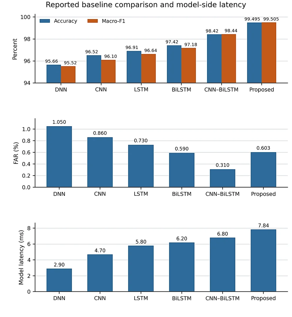
Fig. 5: Baseline comparison. The proposed-model metrics are count-derived from the supplied reference matrix (Class M); the DNN, CNN, LSTM, BiLSTM and CNN–BiLSTM values and the model-side latency are stated comparators (Class R).
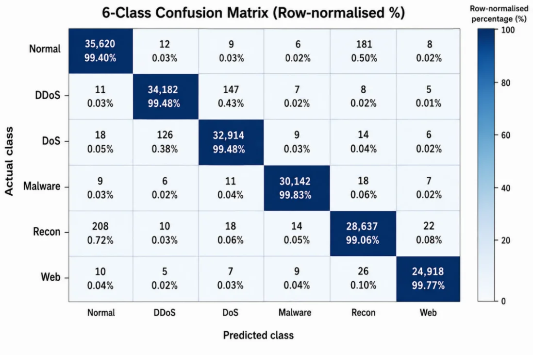
Fig. 6: Supplied pooled reference confusion matrix, N = 187,360 (Class M).
5.2 Cross-dataset transfer
Pooled matrix cannot determine source-only transfer performance. This subsection is thus a distinction between the internal summaries from only stated sources and the balanced transfer reconstructions. The values in Fig. 7 are all Class R and represent intended evaluation settings, not cross-source results.
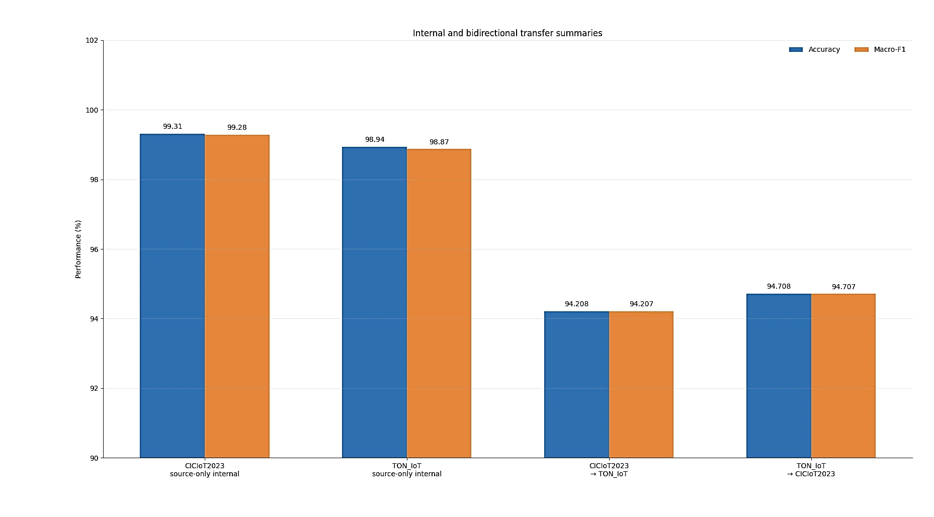
Fig. 7: Stated source-only internal and reconstructed bidirectional transfer summaries (all Class R).
The balanced Class R matrices have macro-F1 values of 94.207% for A→B and 94.707% for B→A, compared with the internal values of 99.28% and 98.87% respectively, as stated in the sources. The differences are 5.073 and 4.163 percentage points respectively. They are 4.663 and 4.573 points higher than the target-only internal values. These are differences in arithmetic, not gaps in generalization measured. The figures are calculated from the tables in Figs. 16 & 17, and each table is divided by the row sum of its actual class in Fig. 9. Normal recall is 95.20% and 95.50%, giving FAR of 4.800% and 4.500%. Precision, recall and F1 are shown in Table 18 assuming the same counts. Within the A→B reconstruction, F1 is lowest for Recon (93.19%), then Web (93.52%) and DoS (93.67%). Within B→A, Recon is lowest (93.82%), followed by DoS (94.16%) and Web (94.21%). Malware is highest at 95.59% and 96.00%. The differences between Malware–Recon are 2.40 and 2.18 points. Recon-to-Normal versus Normal-to-Recon is 3.80% versus 2.10%, and 3.60% versus 2.20%. DoS-to-DDoS is 4.10% and 4.00% respectively, while the other direction is 3.00%. These are characteristics of the matrices assigned, and do not explain the cause of empirical transfer error.
5.2.1 Reconstructed transfer counts and family-level metrics (Class R)
The Class R balanced transfer instances are defined in Tables 16 and 17, with 10,000 windows assigned to each actual class row. These tables are not an independent source, but are used to generate the Fig. 9. The tables give the macro-F1 values that are rounded to 94.207% and 94.707%. They don't get the supports or prediction counts for an executed transfer run. Table 18 and the plotted percentages are derived views of the same instances. The assigned A→B matrix gives accuracy 94.208% and macro-F1 94.207%; B→A gives accuracy 94.708% and macro-F1 94.707%. Their FAR values are 4.800% and 4.500%. These are not independent transfer evidence, but rather views of the same balanced Class R matrices. Recon has the lowest F1 for both Class R transfer instances. Normal→Recon has 210 assigned errors and Recon→Normal has 380 and 360. DoS→DDoS contains 410 and 400. These tables are used to derive all family metrics and plotted confusion percentages; there is no separate source for transfer predictions.
Fig. 8 presents the class-wise cross-dataset transfer performance in both evaluation directions, allowing the family-level precision, recall, and F1 behavior to be compared under the same transfer setting.
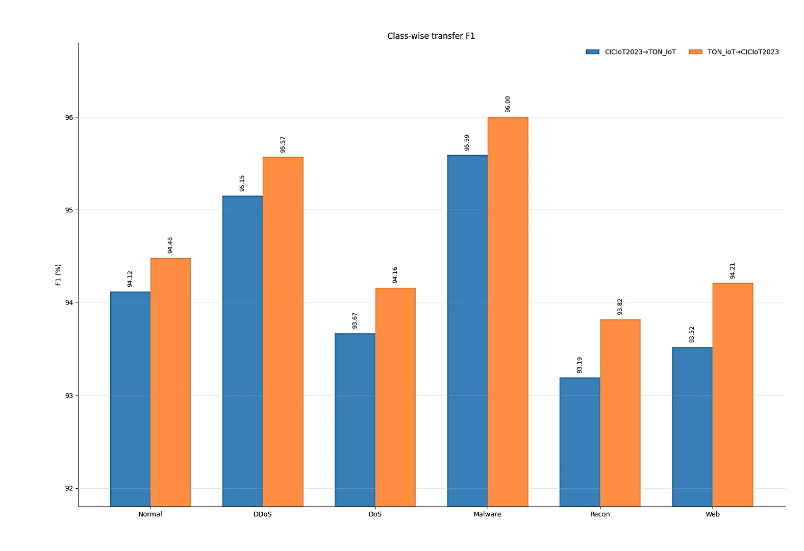
Fig. 8: Class-wise transfer performance in both directions (Class R).
Table 16: Reconstructed A→B counts (Class R); rows are actual classes, columns are predictions
| Actual / predicted | Normal | DDoS | DoS | Malware | Recon | Web |
|---|---|---|---|---|---|---|
| Normal | 9520 | 60 | 45 | 20 | 210 | 145 |
| DDoS | 45 | 9610 | 300 | 15 | 20 | 10 |
| DoS | 65 | 410 | 9320 | 35 | 90 | 80 |
| Malware | 50 | 20 | 45 | 9490 | 120 | 275 |
| Recon | 380 | 65 | 110 | 75 | 9240 | 130 |
| Web | 170 | 35 | 80 | 220 | 150 | 9345 |
Table 17: Reconstructed B→A counts (Class R); rows are actual classes, columns are predictions
| Actual / predicted | Normal | DDoS | DoS | Malware | Recon | Web |
|---|---|---|---|---|---|---|
| Normal | 9550 | 45 | 45 | 20 | 220 | 120 |
| DDoS | 35 | 9650 | 300 | 5 | 5 | 5 |
| DoS | 55 | 400 | 9390 | 25 | 60 | 70 |
| Malware | 55 | 20 | 40 | 9530 | 110 | 245 |
| Recon | 360 | 60 | 100 | 60 | 9300 | 120 |
| Web | 160 | 20 | 70 | 215 | 130 | 9405 |
Table 18. Class-wise metrics derived from the reconstructed counts of Tables 16–17 (Class R), in %.
| Family | A→B P | A→B R | A→B F1 | B→A P | B→A R | B→A F1 |
|---|---|---|---|---|---|---|
| Normal | 93.06 | 95.20 | 94.12 | 93.49 | 95.50 | 94.48 |
| DDoS | 94.22 | 96.10 | 95.15 | 94.65 | 96.50 | 95.57 |
| DoS | 94.14 | 93.20 | 93.67 | 94.42 | 93.90 | 94.16 |
| Malware | 96.30 | 94.90 | 95.59 | 96.70 | 95.30 | 96.00 |
| Recon | 94.00 | 92.40 | 93.19 | 94.66 | 93.00 | 93.82 |
| Web | 93.59 | 93.45 | 93.52 | 94.38 | 94.05 | 94.21 |
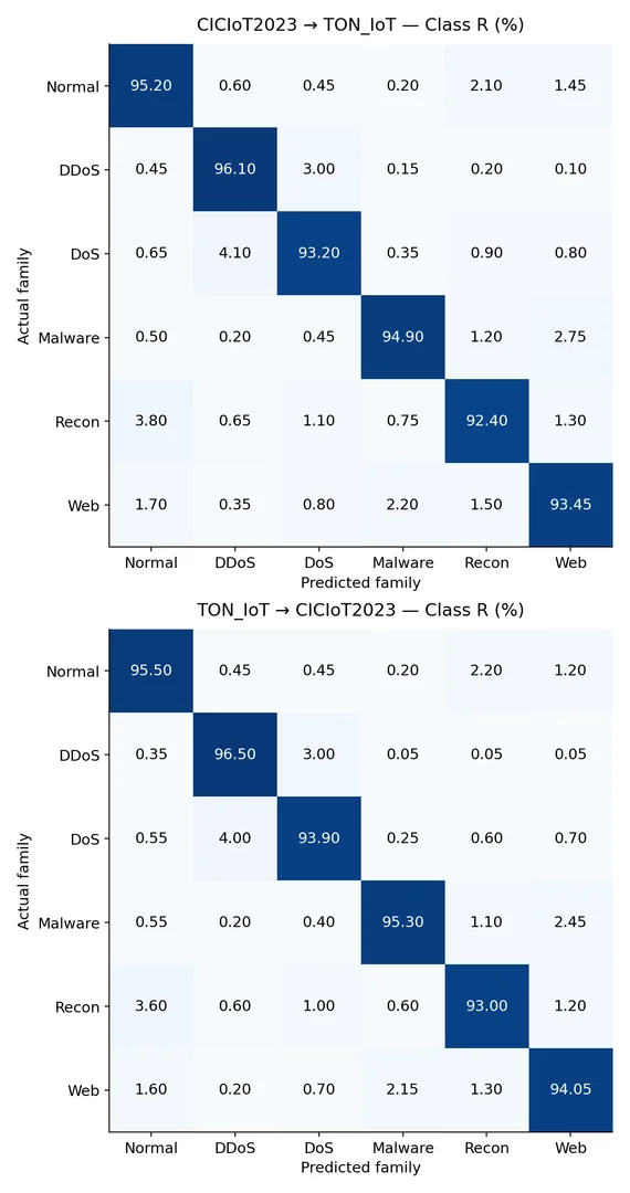
Fig. 9: Row-normalized forms of the balanced Class R matrices in Tables 16–17, in percent.
5.3 Representation ablation and window sensitivity
The following Class R summaries illustrate the intended representation-ablation and window-size comparisons. They do not establish which component caused the reference-matrix result. Post-logit trust controls preserve the argmax labels of fixed logits, so they are evaluated using selective risk and coverage rather than raw class-count gains.
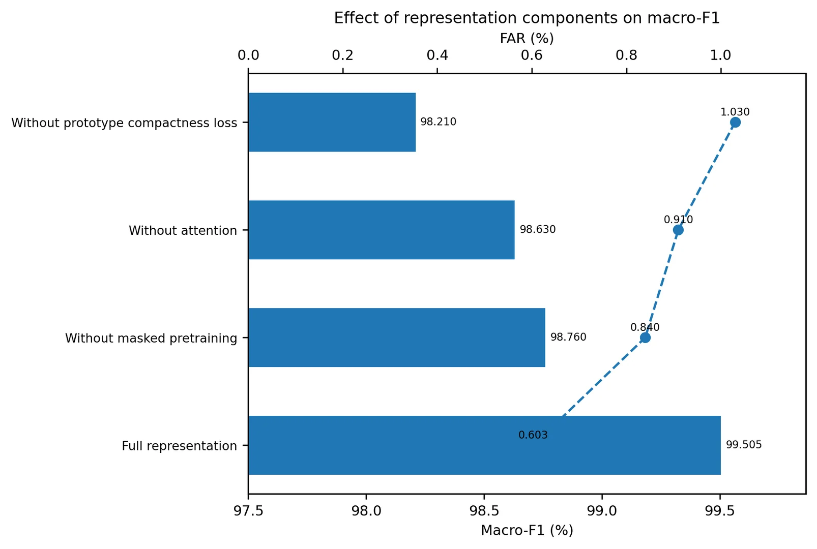
Fig. 10: Stated representation-ablation scenarios (Class R); the full-reference point reuses Class M macro-F1 and FAR.
Fig. 10 summarizes the representation-ablation results and shows the effect of removing individual representation components on macro-F1 and false-alarm behavior. The ablation labels are related to representation learning. If the masked pretraining is removed, only the 8-epoch pretraining is skipped, but the supervised objective (16) remains. If the prototype compactness is removed, its supervised weight is set to zero. These are suggested comparison definitions and are not records of matched training runs. Fig. 11 compares the evaluated window-size settings and illustrates the relationship between temporal context, classification performance, false-alarm rate, and model inference latency. The window-size scenarios with the highest displayed macro-F1 (99.505%) and lowest FAR (0.603%) are T = 10. The T = 5, 15 and 20 F1 values are 98.560%, 99.090% and 98.860%. The difference between the T = 5 and T = 10 is 0.945 percentage points and an assumed model latency of 1.93 ms. T = 20 is assigned 11.24 ms versus 7.84 ms for T = 10. Fig. 12 states a pooled ten-record median span of 1.96 s, IQR 1.31–2.94 s and a 95th percentile (P95) of 5.24 s. These values are an operating point trade-off and not an empirically determined optimum. The reference protocol choice is T = 10 and should be chosen for validation data in an executed study.
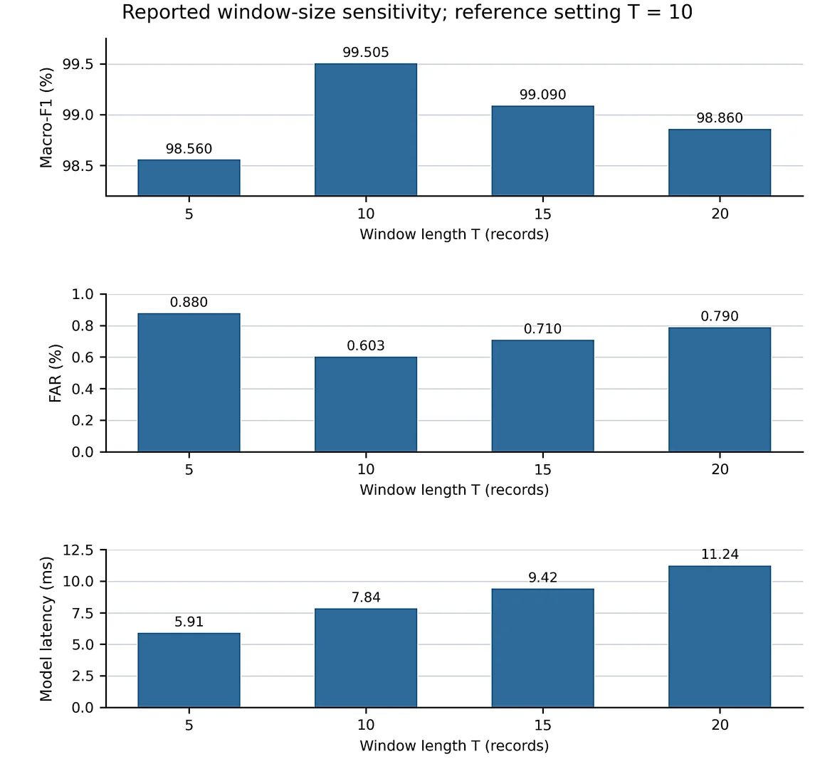
Fig. 11:
Fig. 11: Stated window-size scenarios (Class R); T = 10 reuses Class M macro-F1 and FAR, with Class R latency.
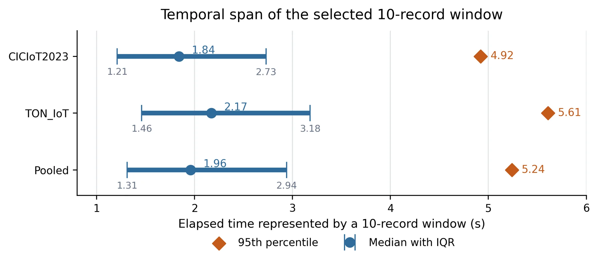
Fig. 12:
Fig. 12: Temporal duration represented by the selected 10-record window (Class R), using the median, interquartile range, and 95th percentile.
5.3.1 Reconstructed window-duration operating points (Class R)
Table 19 is based on the scaling m(T) = 1.96 × T/10 seconds, not on an estimate based on a timestamp. This is an example of a record-count scaling convention. It is different from the exact time interval t_T − t_1 of a realised window, which is not necessarily linearly related to T − 1 successive start-time gaps. Fig. 12 displays independently stated source-specific and pooled quantiles, rather than quantiles reconstructed from raw captures.
Table 19 correlates the performance and model-latency points stated in the window size with the duration convention above. Medians of T = 5, 15 and 20 are scaled linearly according to the given instructions. IQR and P95 are supplied only for T = 10: the pooled IQR is 1.31–2.94 s and P95 is 5.24 s. None of these duration summaries is a measurement from retained timestamps.
Table 19: Illustrative window-size and duration scenarios (Class R); T = 10 F1 and FAR reuse Class M.
| Records | Macro-F1 % | FAR % | Model ms | Median span s |
|---|---|---|---|---|
| 5 | 98.560 | 0.880 | 5.91 | 0.98 |
| 10 | 99.505 | 0.603 | 7.84 | 1.96 |
| 15 | 99.090 | 0.710 | 9.42 | 2.94 |
| 20 | 98.860 | 0.790 | 11.24 | 3.92 |
5.4 Open-set family holdout
Fig. 13 reports the four Class R holdout scenarios under the scope and threshold definitions. The summaries describe unknown recall and known-family retention; they do not represent archived holdout model runs. The holdout rows show that DoS and Recon have lower unknown recall than Malware and Web. This ordering is only an example and cannot provide any overlap between learned families and scores without executed contexts. No round is represented that was held up by DDoS. The four rows of Table 21 are averaged to get unknown recall 93.740%, known macro-F1 98.605%, known false rejection 1.1575% and AUROC 0.96935. These are the arithmetic means of the class R values. Normal and all other known families are known false rejection. Known macro-F1 is not a selective-F1 measure, but is defined on all known test windows prior to rejection.
These scenarios are reproduced in Fig. 14, which is based on the scenarios stated in Table 20. Their AUROCs are 0.9315, 0.9505, 0.9574, 0.9603, 0.9656 and 0.9694 in the displayed method-label order. The combined scenario is 0.76 percentage points higher than the prototype scenario in terms of recall and 0.0038 higher in terms of AUROC. It has four-row mean false rejection of 1.1575%, which is reported as 1.158% in Table 20. This is an ordering that is implied by the illustration and does not mean that an executed scoring method is superior to another.
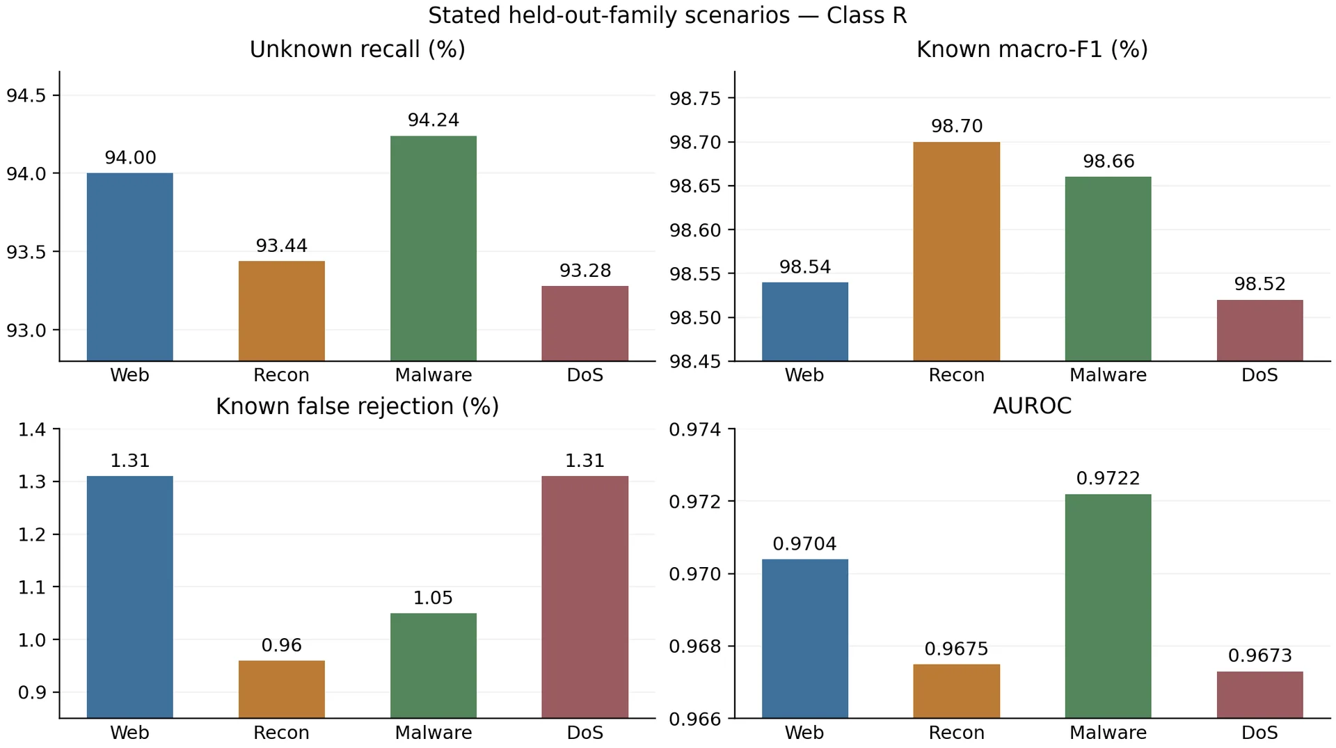
Fig. 13: Leave-one-malicious-family-out unknown-like detection (Class R).
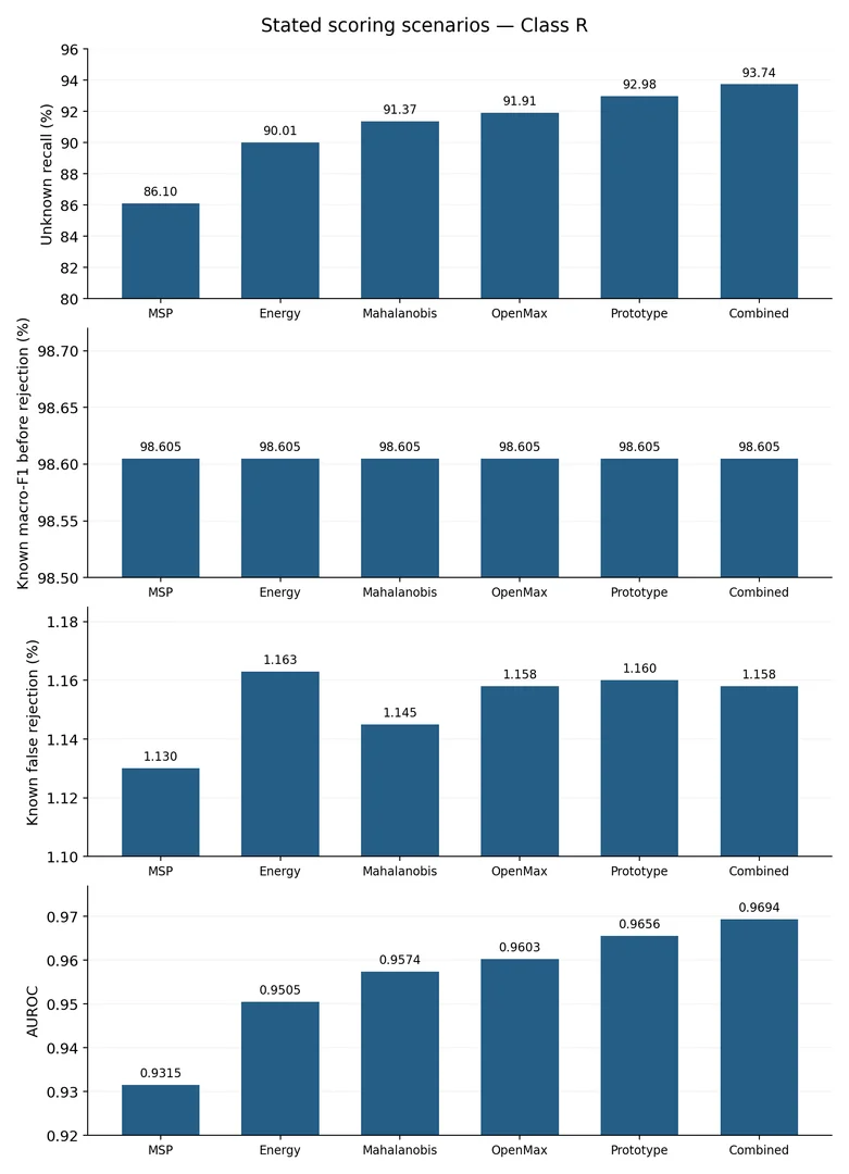
Fig. 14: Open-set comparison across four malicious-family holdouts under the stated score model (Class R).
5.4.1 Rejection-scenario assumptions and interpretation (Class R)
The assigned high-score mixture weights are 0.865, 0.903, 0.918, 0.924, 0.934 and 0.941. If the threshold q is not known, then the unknown recall at threshold q would be w•Pr(S_high > q) + (1 − w)•Pr(S_low > q). Not all weight is equal in determining that recall or AUROC. The weights displayed are a general approximation of the weights, but the missing component distributions do not allow exact regeneration or verification of the claimed mixture origin. Method labels are not used to denote algorithms that are actually executed. The comparative claim is open as the method labelled scores are not retained on common per window activations. They are to be evaluated for their ordering as outlined.
Table 20: Score-distribution comparison under the stated score model (Class R), averaged across four rounds
| Assigned scenario | Unknown recall % | Known F1 % | False rejection % | AUROC |
|---|---|---|---|---|
| MSP | 86.10 | 98.605 | 1.130 | 0.9315 |
| Energy | 90.01 | 98.605 | 1.163 | 0.9505 |
| Mahalanobis | 91.37 | 98.605 | 1.145 | 0.9574 |
| OpenMax | 91.91 | 98.605 | 1.158 | 0.9603 |
| Prototype | 92.98 | 98.605 | 1.160 | 0.9656 |
| Prototype + uncertainty | 93.74 | 98.605 | 1.158 | 0.9694 |
Table 21: Combined-score results by withheld-family label under the stated score model (Class R)
| Family | Unknown recall % | Known F1 % | False rejection % | AUROC |
|---|---|---|---|---|
| Web | 94.00 | 98.54 | 1.31 | 0.9704 |
| Recon | 93.44 | 98.70 | 0.96 | 0.9675 |
| Malware | 94.24 | 98.66 | 1.05 | 0.9722 |
| DoS | 93.28 | 98.52 | 1.31 | 0.9673 |
The assigned high-score mixture weights are 0.865, 0.903, 0.918, 0.924, 0.934 and 0.941. Unknown recall at threshold q would equal w·Pr(S_high > q) + (1 − w)·Pr(S_low > q). A weight alone does not determine that recall or AUROC. The displayed recalls broadly track the weights, but the missing component distributions prevent exact regeneration or verification of the claimed mixture origin. Method labels identify scenarios, not executed algorithms. The comparative claim remains open because the method-labelled scores have not been retained on common per-window activations. specifies the evaluation needed to test their ordering.
5.5 Calibration and selective trust
Tables 22–24 present the Class R calibration and acceptance scenarios with the fixed reference-matrix counts. The questions answered by full-population probability and accepted-only error are different, as explained in 4.5 and 4.5.1. The raw class predictions are preserved with positive temperature scaling. The effect of its illustrated must therefore be evaluated using probability metrics, and the gate using error and coverage of accepted decisions. The Class R summaries are based on the following constraints: The 187,360 window matrix and accuracy 0.994946. Probability bounds and accepted-error arithmetic can be verified, but the original logits, construction code and acceptance ranks are not available. These aggregates do not provide an acceptable probability and acceptance ledger. The next analysis is used to check the necessary consistency conditions of the aggregates. Does not rebuild missing per-window probability and acceptance records.
5.5.1 Calibration consistency and accepted-error analysis (Class R)
The probability illustration keeps all the argmax counts of each class in the Class M matrix. The method for determining its probability and acceptance outputs is described and this analysis only considers the aggregates shown. The stated temperature is displayed below, with a different window length T than the validation window length τ, which is required for the fitting procedure. The value is thus a Class R input and not an independently verified fitted value.
τ = 1.103552 (37)
In the range of values given, ECE and NLL are decreasing and Brier is slightly increasing. The accuracy is still the matrix-derived one, before/after is the same. Both shown ECE values are below the upper bound and the lower bound |accuracy − mean confidence| ≤ ECE is met. These checks are not meant to imply that each entry was generated from these logits.
ECE ≤ (1 − accuracy) + (1 − mean confidence) (38)
Coverage = accepted / N Selective risk = accepted errors / accepted (39)
Table 22: Stated probability-calibration summaries (Class R), not recoverable from the matrix alone.
| Metric | Before temperature | After temperature |
|---|---|---|
| Accuracy, fraction | 0.994946 | 0.994946 |
| Mean maximum confidence | 0.996977 | 0.994222 |
| ECE, 15 bins | 0.002044 | 0.000724 |
| Multiclass Brier | 0.010100 | 0.010125 |
| Negative log-likelihood | 0.043029 | 0.042056 |
| ECE upper bound | 0.008077 | 0.010832 |
Table 23: Stated risk–coverage operating points (Class R); full-coverage counts derive from the reference matrix
| Coverage % | Accepted | Deferred | Accepted errors | Risk % | Accepted FAR % |
|---|---|---|---|---|---|
| 100.000 | 187360 | 0 | 947 | 0.5054 | 0.6027 |
| 99.000 | 185486 | 1874 | 596 | 0.3213 | 0.3920 |
| 97.000 | 181739 | 5621 | 420 | 0.2311 | 0.2905 |
| 95.000 | 177992 | 9368 | 334 | 0.1876 | 0.2410 |
| 90.000 | 168624 | 18736 | 206 | 0.1222 | 0.1490 |
Table 24: Stated gate scenarios at 95% coverage (Class R)
| Gate scenario | Accepted | Accepted errors | Risk % | Accepted FAR % |
|---|---|---|---|---|
| Confidence only | 177992 | 900 | 0.5056 | 0.6186 |
| Prototype scenario | 177992 | 613 | 0.3444 | 0.4410 |
| Combined scenario | 177992 | 334 | 0.1876 | 0.2410 |
Test labels are not allowed in an executed study with acceptance ranking. Here, the confidence-only illustration is near the random-deferral expectation 0.05 × 947 = 47.35 of errors deferred at 95% coverage. This is not a proof of its randomness or of its lack of discriminatory power. The total number of accepted errors (assumed) is 334 in the combined scenario. Partial-coverage FAR entries cannot be independently recomputed because the numerator and denominator counts of accepted FAR are not available. The operating points are not validated results from a validation selected deployment threshold.
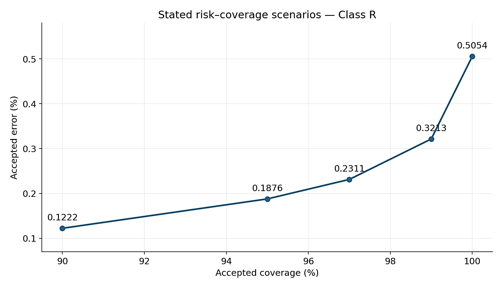
Fig. 15: Stated accepted-error and coverage scenarios (Class R), with risk computed from Table 23.
The combined-gate scenario assigns fewer accepted errors than the confidence-only scenario at the same stated coverage. This is the contrast the matched protocol must test; the assigned counts do not establish that the proposed gate generated the ranking. Representation ablation and gate ablation remain separate because the latter holds raw predictions fixed.
5.6 Controlled drift
The assigned PSI/JSD examples are correlated with the declared state thresholds. They show the classification of monitors and proposed routing responses, rather than any observed changes from retained reference and perturbed streams. Empirical monitor sensitivity and delay are not measured.
The illustrative logit-noise scenario is shifted, with JSD of 0.083. Input PSI is not shown in the figure because it is not a change that is measured separately. The other pairs of assigned PSI/JSD also adhere to the threshold rules. Stable, warning and shifted states are used to route, and all relevant disruption guards are still mandatory. Workload, detection delay or network-risk-reduction are not measured in these examples.
JSD = 0.083 > 0.05 (40)
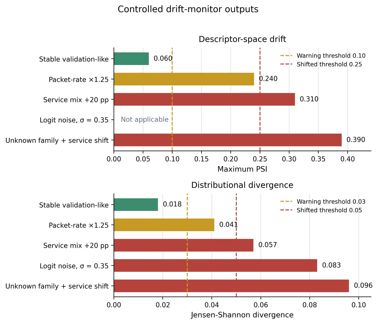
Fig. 16: Controlled PSI and JSD drift-monitor outputs under the stated shift scenarios (Class R); colours identify stable, warning, and shifted states.
5.7 Policy stress test
The fixed-state simulator now shows how hard constraints can prevent a candidate from being selected even though they have a lower simulated next risk. The outputs are derived from the inputs provided in Tables 9 and 10, and are independent of the Class R classifier and gate summaries.
Table 25 shows the tested candidate's response and the selected response. The simulated next risk for candidate blocking is 0.1729 in the Recon/Normal boundary state while the simulated next risk for the selected review action is 0.4249. The ambiguity rule is not followed even though it has a lower simulated risk. In unknown-like shifted state, candidate allow has next risk 0.8648 and is rejected, whereas review is the lowest-objective admissible action, with next risk 0.6218. The utility objective and hard constraints are therefore the two factors that govern the scenario routing.
Table 25: Candidate actions, hard-rule decisions, and selected simulator risk (Class A)
| Scenario | Candidate | Simulated next risk | Rule result | Selected action |
|---|---|---|---|---|
| Stable Normal | allow | 0.1234 | Accept Rule 1 | allow (0.1234) |
| DDoS, high confidence | allow | 0.9386 | Reject Rule 2 | block (0.2411) |
| Malware, close prototype | monitor | 0.7544 | Reject Rule 3 | isolate (0.1384) |
| Recon/Normal boundary | block | 0.1729 | Reject Rule 4 | review (0.4249) |
| Unknown-like and shifted | allow | 0.8648 | Reject Rule 5 | review (0.6218) |
The same linear clipped transition in Eqs. is used in Fig. 17. (26) and (30), with the utility in Eqs. (27) and (31). The pre-action to selected-action risk pairs are 0.1200→0.1234, 0.9300→0.2411, 0.8800→0.1384, 0.5600→0.4249 and 0.8100→0.6218. Their signed differences are −0.0034, 0.6889, 0.7416, 0.1351 and 0.1882. They are not measured reductions in network risk, but rather deterministic consequences of assigned scenario values and admissible sets.
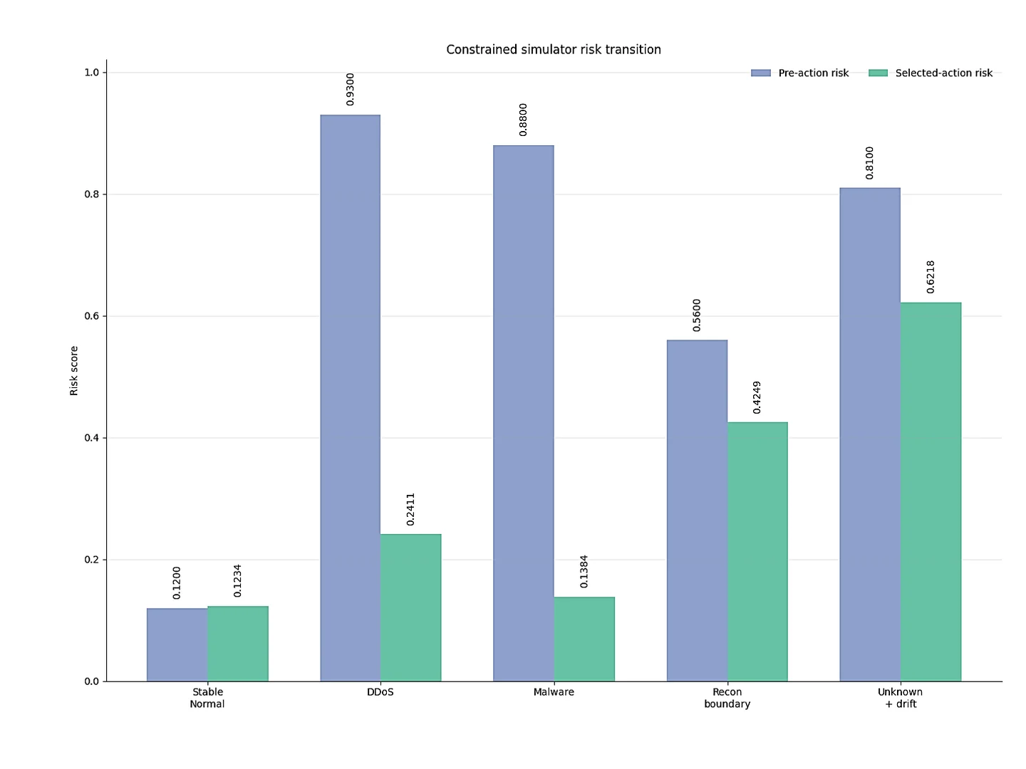
Fig. 17: Pre-action and selected-action risk in the five policy stress scenarios (Class A).
5.7.1 Fixed-state outputs and stated sensitivity
Table 26 is Class A: each selected action, risk and objective is a consequence of the given fixed inputs. Table 27: Class R: its random-perturbation summary does not contain a retained draw ledger or random seed. There is no evidence in either table of the outcomes of the causal network.
Table 26: Simulator outputs computed from the specification (Class A)
| State | Selected action | Next risk | Objective | Risk difference |
|---|---|---|---|---|
| Stable Normal | allow | 0.1234 | 0.1234 | -0.0034 |
| DDoS | block | 0.2411 | 0.2555 | 0.6889 |
| Malware | isolate | 0.1384 | 0.1834 | 0.7416 |
| Recon boundary | review | 0.4249 | 0.4537 | 0.1351 |
| Unknown + drift | review | 0.6218 | 0.6470 | 0.1882 |
Table 27: Stated sensitivity summary for ±20% coefficient perturbations (Class R).
| State | Same action % | 2.5% next-risk quantile | 97.5% next-risk quantile |
|---|---|---|---|
| Stable Normal | 25.55 | 0.0807 | 0.1238 |
| DDoS | 100.00 | 0.1099 | 0.3730 |
| Malware | 100.00 | 0.0063 | 0.2794 |
| Recon boundary | 100.00 | 0.3926 | 0.4578 |
| Unknown + drift | 100.00 | 0.5729 | 0.6702 |
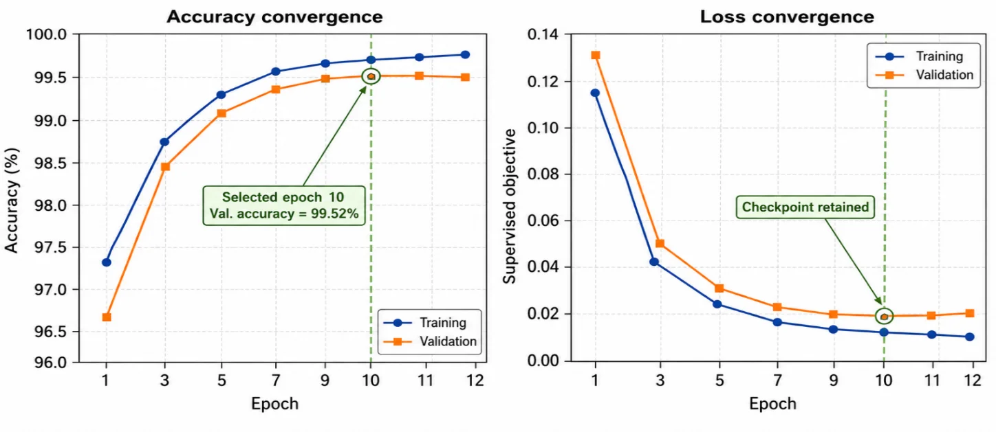
Fig. 18: Stated convergence trajectory with an illustrative Epoch 10 selection point (Class R).
The retained sensitivity summary is a description of 2,000 independent uniform multiplicative perturbations per state, over action effects, disruption costs and the uncertainty/drift coefficients, with effects clipped to [0,1]. Random seeds, generator state and draw ledger are not available, so the quantiles and same-action frequencies listed cannot be reproduced exactly. These are illustrative sensitivity values and not confidence intervals or an independent check of Table 26. The 25.55% stable-Normal figure is not a measured stability rate, but rather a motivator for a future sensitivity study. With the current admissible sets, both Malware and unknown-plus-shift have one action, and by definition 100% action retention is guaranteed in those scenarios. Observed interventions or an independently specified network emulator would be needed for independent policy validation. A second set of data based on the same risk equation would not be independent. The open-set ordering and the seed differences are Class R and are not providing that independence.
5.8 Training convergence and multi-run stability
This subsection distinguishes a stated convergence trajectory and a series of seeds from the test metrics derived from the count. No training run is identified by any of the curves or seed labels. The following arithmetic shows the way they are supposed to report.
Table 28: Reference discrimination and stated loss/convergence values. Test accuracy and macro-F1 are Class M; all other cells are Class R
| Stage | Accuracy (%) | Macro-F1 (%) | Supervised loss |
|---|---|---|---|
| Training | 99.70 | 99.68 | 0.0134 |
| Validation | 99.52 | 99.50 | 0.0191 |
| Test reference: M metrics / R loss | 99.495 | 99.505 | 0.0198 |
The differences between training and test accuracy and macro-F1 are 0.205 percentage points and 0.175 points, respectively, as stated in Table 28. The difference in test and validation loss is 0.0007. These are arithmetical differences between values derived from the matrix and illustrative values, not evidence of overfitting. The loss column is an illustrative supervised loss series, not the full regularized objective nor the NLL series in Table 22; the missing training and probability logs make it impossible to link these two series. Fig. 18 is an illustrative reference checkpoint for epoch 10. That illustration shows the label “retained” for the assigned selection point, which is not a trained checkpoint. The rule used is the one which gives the highest validation accuracy in full precision, patiently, with patience 3 and 12 epochs limit. The curve is merely illustrative and does not indicate which stopping condition would be reached in a run that was executed.
The displayed trajectory is illustrative. Neither its train/validation separation nor its assigned checkpoint verifies convergence, validation saturation, generalization or the absence of leakage.
$95% CI = 99.490 pm 2.776 imes rac{0.031623}{sqrt{}5} = lbrack 99.451,99.529 brack%$ (41)
5.8.1 Paired-run statistical procedure on a stated series (Class R)
Class R is the ten-value series and is used for the paired-testing arithmetic. The CNN–Transformer column is not a baseline trained with Table 11, but rather an additional illustration of a classifier. The nearest-prototype classifier is different from the prototype rejection gate of Table 14, which keeps the label, and assigns the closest prototype label. This separation allows for different values of F1 to be obtained without assigning raw-F1 changes to a post-logit gate. There are no training runs recorded in any of the columns. The difference between percentage valued metrics and their intervals are reported in percentage points (pp). The ten stated values have mean 99.490%, sample SD 0.025820 percentage points and a two-sided t-interval of [99.472, 99.508]%. The five main values are in a precise sequence of 0.02 points. This regularity is not a characteristic of the assigned series, but rather an indication of independent seeded optimization.
Table 29: Stated macro-F1 series used to specify the paired procedure (Class R), in %
| Seed | Proposed | CNN–BiLSTM | CNN–Transformer | Nearest-prototype classifier |
|---|---|---|---|---|
| 11 | 99.45 | 98.38 | 98.65 | 99.31 |
| 23 | 99.47 | 98.42 | 98.69 | 99.35 |
| 37 | 99.49 | 98.47 | 98.73 | 99.37 |
| 51 | 99.51 | 98.40 | 98.66 | 99.34 |
| 71 | 99.53 | 98.49 | 98.76 | 99.40 |
| 89 | 99.48 | 98.43 | 98.70 | 99.36 |
| 103 | 99.50 | 98.46 | 98.74 | 99.38 |
| 127 | 99.46 | 98.37 | 98.64 | 99.33 |
| 149 | 99.52 | 98.51 | 98.78 | 99.41 |
| 173 | 99.49 | 98.45 | 98.71 | 99.35 |
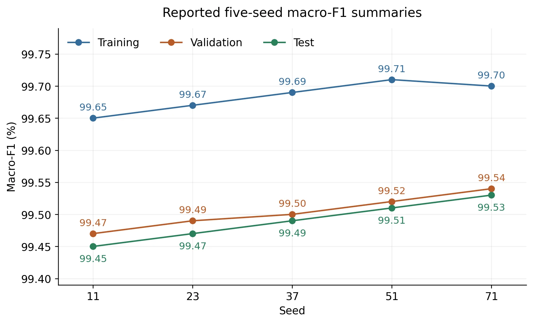
Fig. 19: Macro-F1 dispersion across the five primary seed labels of the stated series (Class R).
Fig. 19 presents the corresponding response-control results and illustrates how the decision policy behaves under the evaluated operating conditions.
Table 30: Paired analysis computed from the stated series of Table 29 (Class R)
| Comparator | Mean difference, pp | 95% t-interval, pp | Exact p | Holm p |
|---|---|---|---|---|
| CNN-BiLSTM | 1.052 | [1.030, 1.074] | 0.001953 | 0.005859 |
| CNN-Transformer | 0.784 | [0.761, 0.807] | 0.001953 | 0.005859 |
| Nearest-prototype classifier | 0.130 | [0.118, 0.142] | 0.001953 | 0.005859 |
The two-sided sign-flip calculation counts the number of ways the signs can be assigned to the ten paired differences, which is 1,024. All three constructed comparisons have the same smallest attainable two-sided value shown below. The three tied comparisons are 0.005859375 after being adjusted for Holm. At n = 10 the smallest possible two-sided result of the sign-flip calculation is 2/1024, and three comparisons that are tied at that floor provide no information about the relative strength of the two. The calculation is not meant to be used to make a comparison, but rather to report the procedure.
$p = rac{2}{1,024} = 0.001953125$ (42)
To make a true inference, paired runs must be the same split and seed definition, and the exchangeability assumptions of the test must be justifiable. Variability of seeds within one fixed split does not imply uncertainty at sites, capture days or datasets. The first statistical item of future work is to perform the ten matched-seed runs for the proposed model and each comparator and then to recompute Table 30 from the outputs retained from each of these runs.
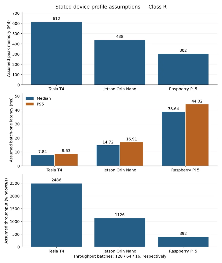
Fig. 20: Gateway profiling values under the stated device profile (Class R); these are the device-specific inputs to the Class A budget of Table 31. Analytical MAC/FLOP quantities are specified separately.
5.9 Deployment resource and gateway profiling
This section is about whether it's possible to produce the decision in time and within the memory of a gateway-class device; the preceding subsections are about what the framework decides. Model-side cost and end-to-end budget are reported separately as they have different bounds. Fig. 20 contains Class R device-profile assumptions: batch-one median/P95 latency of 7.84/8.63 ms for Tesla T4, 14.72/16.91 ms for Jetson Orin Nano and 38.64/44.02 ms for Raspberry Pi 5; peak memory of 612, 438 and 302 MB; and throughput of 2,486, 1,126 and 392 windows/s at batches 128, 64 and 16. The training time assumption for T4 is 41.7 min. These are not device measurements validated. The batch throughput is different from the batch-one latency. These assumed model-side values do not include capture, extraction, communication, enforcement and analyst delay. The number of trainable parameters is 756,486 as shown in Table 32. Raw 32-bit floating-point (FP32) weights occupy 3.025944 MB (2.885765 MiB). This is not a checkpoint-file size, but rather the size of the file before gradients, BatchNorm state and serialization overhead are included, which is 9.077832 MB. The affine CNN, BiLSTM and attention components need 309,120, 6,553,600 and 657,920 multiply–accumulate operations (MACs), respectively, or 7,520,640 multiply/add operations. The addition of attention context aggregation brings 2,560 MACs. Selected arithmetic and special-function work are listed separately in Fig. 22, but this is not a complete runtime graph profile.
5.9.1 Analytical sequential deployment budget (Class A)
The class of Table 31 is A. It calculates the latency budget of Eq. (43) from the given per-stage latency values, and sums up the latencies arithmetically. The window-accumulation term is the 10-record term and the analyst term is a specified review delay of 26,000 ms, which are not executed measurements.
Table 31: Sequential latency budget composed from stated stage values (Class A), all values in ms.
| Stage | Tesla T4 | Jetson Orin Nano | Raspberry Pi 5 |
|---|---|---|---|
| Window accumulation | 1960.00 | 1960.00 | 1960.00 |
| Preprocessing | 0.84 | 1.46 | 3.86 |
| Queue delay | 0.31 | 0.64 | 1.25 |
| Model inference | 7.84 | 14.72 | 38.64 |
| Communication | 1.42 | 1.73 | 2.17 |
| Enforcement | 0.76 | 1.12 | 1.94 |
| Automatic total | 1971.17 | 1979.67 | 2007.86 |
| Review-path total | 27971.17 | 27979.67 | 28007.86 |
The review path is an additional 26,000ms analyst delay on the automatic path. The model-only medians of 7.84, 14.72 and 38.64 ms are used as device-specific inputs. Window accumulation is the dominant factor in the budget, on all devices, and model-side latency is not the limiting factor on end-to-end response time. Overlapping capture and processing must be modelled separately in a streaming deployment. The following properties should be recorded in an executed profile: device model, power mode, clocks, runtime version, precision and batch size. It should run 200 warm-up iterations and 2,000 iterations in the batch mode and keep per-iteration latency and memory logs for median/P95 summaries. These settings set up the future measurement procedure. Fig. 20 is not provided with such logs or several details of device configuration.
6. Discussion
The results can be used to support three different conclusions. First, the reference matrix shows that there are concrete error concentrations, Recon-to-Normal confusion is more common than the other direction, so per-family analysis is needed in addition to macro-F1. Second, the analytical policy scenarios reveal that response constraints may rule out a lower-risk simulated candidate; the chosen action is both admissible and useful. Third, the illustrative transfer, rejection and gate summaries specify the comparisons needed to assess the proposed interface but do not provide an empirical ordering of the comparisons. The main outstanding issue is whether the trust gate improves the acceptance of errors at similar coverage and whether the response constraints enhance admissibility at a reasonable review burden. The matched evaluation for that question is
defined.
6.1 Threats to validity
Internal validity. The group assignment before fitted transforms and window construction is not a property of the provided matrix, but a protocol requirement. It needs to be audited, and for that, capture provenance, group keys, duplicate checks, split manifests, checkpoint identifiers and validation-selection records are needed. Leakage control and a training history cannot be set up with matrix arithmetic. Construct validity. The six umbrella families are a compacting of heterogeneous attack mechanisms. Malware-level transfer does not create transfer between all constituent subtypes. FAR is based on real Normal windows and the holdout rejection is for the unseen benchmark families, not universal zero-day detection. PSI and JSD measure monitored distribution differences, not attack intent. External validity. There are two lab benchmarks that do not cover the operational range of IoT. TON_IoT is an IoT/IIoT scenarios set in TON_IoT, which does not imply performance in an arbitrary industrial, medical or home deployment. Local traffic, calibration, thresholds and service policies need to be evaluated separately. Statistical conclusion validity. The intervals obtained in the above are for the seed series Class R and not for optimisation variability of an executed model. This paper does not make any claim to statistical superiority over any baseline. Simulator validity. The fixed-state results are obtained from the coefficients assigned and admissible sets of actions. They do not have an independent network validation. The sensitivity table is not a calculation that can be reproduced from a fixed set of inputs, but rather a summary of random perturbations stated.The sensitivity table is not a calculation that can be reproduced from a fixed set of inputs, but rather a summary of random perturbations stated.
6.2 Deployment boundary
The deployment relation below is used to split the latency stages. The other device profiles are Class R assumptions, with the 7.84 ms T4 model value. They are not a guarantee of model portability, real-time
suitability or end-to-end response time on measured hardware when used in the analytical budget.
Ltotal = Lcapture + Lfeature + Lqueue + Lmodel + Lcommunication + Lenforcement + Lhuman (43)
The proposed deployment role is Gateway Decision Support. Stable supported predictions may allow for bounded automatic action only under applicable guards, ambiguity and shift and critical-service restrictions result in review. Memory admission is confirmed by the analysts, and it is still separate. Evaluations of the devices and networks are required to be performed to determine feasibility, profiling accuracy and actual response time.
6.3 Decision acceptance, coverage, and audit trail
The framework’s operational output should be evaluated as a selective decision system. Let qi = 1 when a window passes the calibration, prototype, drift, and rule gates and qi = 0 when it is deferred. Decision coverage and selective error are
$Coverage = rac{1}{n}sum_{i}^{}q_{i},quadquad{Risk}_{sel} = rac{sum_{i}^{}q_{i}mathbf{1}leftlbrack {widehat{y}}_{i} eq y_{i} ight brack}{sum_{i}^{}q_{i}}.$ (44)
Coverage is the percentage of windows that the gate will accept. Selective risk is the error fraction of the windows accepted and is defined only if A = ∑ᵢqᵢ > 0. It is undefined at zero coverage. Equations (44) and (47) are thus written with the same denominator of accepted counts, but no additive constant. The pooled confusion matrix has 187,360 windows, and 947 classification errors, resulting in a full-coverage error rate of 0.505444%. The notation and range of the following bounds are defined below.
N = 187, 360, E = 947, 0 < A ≤ N (45)
max(0, E − (N − A)) ≤ EA ≤ min(E, A) (46)
$ rac{max(0, E - (N - A))}{A} leq Selective risk leq rac{min(E, A)}{A}$ (47)
The selective-risk bounds are Class A, conditional on the provided N and E. The accepted-error scenarios, holdout AUROC 0.9694 and mean known false rejection 1.16% are Class R, which together represent a reporting interface, rather than the performance of a deployed gate.[29] A decision record associates the window and group identifiers with the model version, predicted family, calibrated confidence, entropy, margin, prototype distance and monitored shift state. It also documents candidate utilities, rejected constraints, the action selected and disposition by the analyst. The operating point is determined by the validation, which is performed under the given false-alarm and service constraints. Test coverage is an outcome rather than a tuning criterion. The gate differentiates between representation-based rejection, ambiguity-based deferral and operational deferral. These causes are not mutually exclusive: A small class margin cannot be overcome by adequate prototype support, and agreement of statistical signals cannot supersede a critical-service restriction. Decision acceptance can be judged independently of raw classification in the case of separate routing reasons.
6.4 Computational and governance boundary
The affine CNN, BiLSTM and attention subtotal is 7.520640 million MACs, which is 15.041280 multiply/add operations. The Context aggregation contributes 0.002560 million MACs. The input scaling requires about 660 scalar operations for 10 x 33 values. The scalar-dispersion prototype distance in Eq. (19) requires 4,608 arithmetic operations and six square roots in six 256-dimensional contexts, apart from CDF lookup and comparisons. There are five candidate actions and seven rules, which provide at most 35 action–rule predicate evaluations. Without the drift histogram, there is no exact monitor operation count inferred, and the costs of drift histogram depend on the binning and implementation.
6.4.1 Analytical parameter and selected-operation inventory (Class A)
Table 32 provides an exact calculation of the parameters for the given inference architecture. Fig. 22 provides an example of an arithmetic inventory (under an explicit counting convention) rather than a full implementation-independent FLOP count. Memory movement, comparisons, lookup, histogram updates and runtime scheduling are outside that inventory.
The specified graph contains 756,486 trainable parameters and 384 non-trainable BatchNorm values. FP32 storage for both is 3.02748 MB, excluding prototypes, scalers, activations, allocator overhead and file-format metadata.
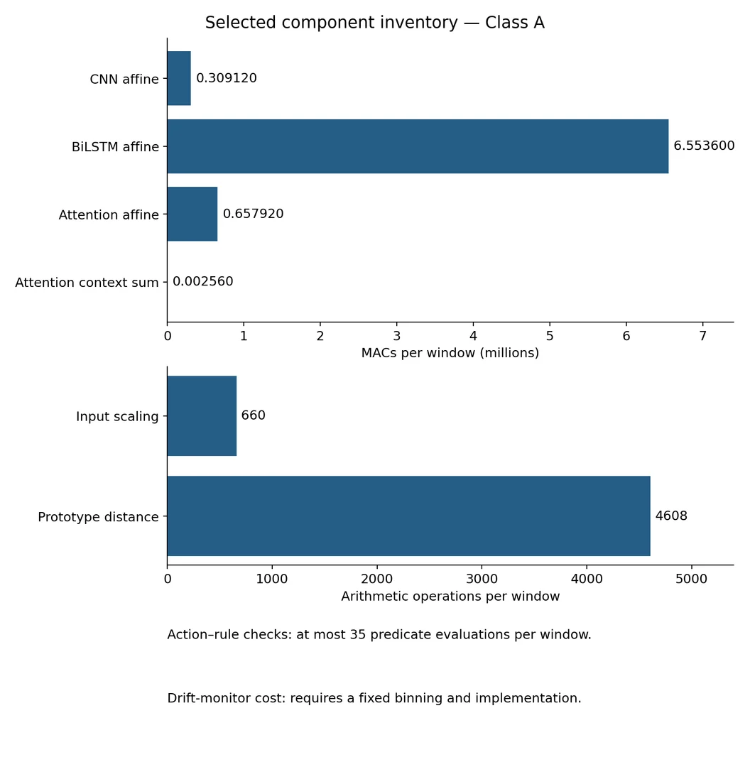
Fig. 21: Selected component costs (Class A), with MACs, scalar operations and predicate checks kept separate.
Table 32: Parameters of the specified inference architecture (Class A).
| Component | Trainable parameters |
|---|---|
| Conv1 | 6,400 |
| Conv2 | 24,704 |
| BatchNorm trainable | 384 |
| BiLSTM layer 1 | 263,168 |
| BiLSTM layer 2 | 394,240 |
| Additive attention | 66,048 |
| Classifier | 1,542 |
| Total | 756,486 |
| BatchNorm non-trainable state | 384 |
The selected inventory totals 15.107943 million arithmetic operations, with multiplication and addition counted separately. The count includes CNN and recurrent affine work, attention projection and context aggregation, classifier affine work, biases, LSTM state arithmetic, four scalar BatchNorm operations per activation with cached denominators, input scaling, scalar-dispersion prototype distances, two softmax normalisations, temperature division, entropy, margin and the weighted rejection sum. An additional 30,108 special-function evaluations comprise 25,600 LSTM sigmoid/tanh, 1,920 GELU, 2,560 attention tanh, 16 exponentials, six logarithms and six prototype square roots. Protective entropy additions are counted. Comparison instructions, clipping, distance-CDF lookup, quantile fitting, histogram updates, decoder training and runtime overhead are excluded.
This is a specified counting convention rather than a profiler output. Device assumptions remain Class R; the arithmetic inventory cannot validate those timings.
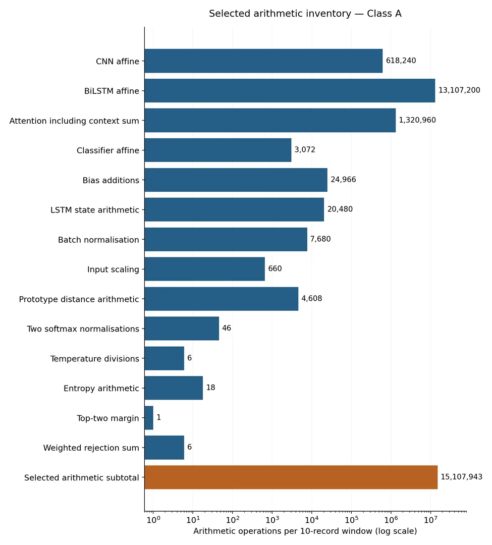
Fig. 22: Selected arithmetic-operation inventory for the specified 10-record inference path (Class A).
6.5 Records required for reproducibility
Records need to be maintained at the claim level in order to reproduce. The reference counts and class order are required for matrix derived metrics. The inputs, architecture and counting convention are required for analytical policy and resource calculations. Empirical evaluation additionally needs capture/label manifests, group assignments and splits, versioned extractor and decoder code, fitted transforms and prototypes, checkpoints, calibration logits and fitting traces, per-window scores and acceptance decisions, accepted-Normal supports, drift histograms and binning, and device configuration and timing logs. Random-sensitivity results require the generator, the seeds and the retained draws. The tables provided can be used for the first two types of arithmetic; the missing empirical records cannot be recovered from the counts.
7. Limitations and future work
The primary drawback is that the Class R summaries are not linked to the actual experiments that were performed. The evidence boundaries and specific threats to validity are specified. The first step in validation is to establish capture provenance and group-isolate splits, followed by the source-only transfers and matched rejection and gate comparisons. It is important to keep per-window outputs before estimating variability between training seeds or profiling devices. Further research needs to explore a DDoS holdout, natural target prevalences, independent capture environments, and chronological drift and longitudinal memory. Assigned simulator effects are not measured intervention effects, so response outcomes need to be assessed at the network level.
8. Conclusion
CNS-STGU Defense sets up a trust-conditioned basis for intrusion decision support of IoT in which the intrusion class prediction, evidence acceptance and response admissibility are considered as independent yet interrelated steps. This separation is important because the primary drawback of score-based intrusion detection is that a high confidence label does not imply that the traffic is backed by the learned representation, is within the monitored distribution, or allows for an automated response. At the classification layer, the supplied 187,360-window reference matrix yields 99.495% accuracy, 99.505% macro-F1, an MCC of 0.9939, and a FAR of 0.603%. The balanced bidirectional transfer reconstruction results are macro-F1 94.207% and 94.707%, respectively, which is 4.798-5.298 percentage points lower than the pooled internal results. This gap is a measure of the impact of the source change, and demonstrates the need for external accuracy to be used as the basis for deployment claims. In addition to aggregate classification metrics, family-level confusion, false rejection, decision coverage and accepted-decision risk should be reported. The primary contribution is an auditable decision pathway that is constructed from a 33-descriptor common representation, group-isolated partitioning, a CNN-BiLSTM-attention encoder, calibrated confidence, entropy, class margin, prototype support, PSI/JSD drift monitoring and constraint-governed response selection. The framework documents the reasons for accepting, deferring or rejecting a prediction and for admitting or blocking a candidate response. It also sets matched comparisons with known rejection techniques and distinguishes between model error and operational load caused by deferral and analyst review. The study offers a repeatable specification for assessing IoT intrusion detection with accuracy other than the benchmark. It is a numerical audit, explicit evidence classes, selective-risk formulation and resource inventory that spell the evidence needed to get from classification performance to accountable gateway decisions. The other empirical requirement is to perform the matched cross-dataset, unknown-family, calibration, drift and constrained-response tests with retained per-window outputs, fitted artefacts, split manifests, timing logs and response records. The combined trust gate's ability to reduce error for accepted decisions at similar coverage and the ability of constrained actions to be accepted under realistic IoT traffic and service conditions will be determined by completing this validation.
Funding Declaration
This research did not receive any specific grant from funding agencies in the public, commercial, or not-for profit sectors.
Data Availability Statement
The datasets used in this study are publicly available from their original sources, including CICIoT2023 and TON_IoT. The processed validation data, feature-mapping specifications, experimental configurations, and source code used to support the reported analysis are available from the corresponding author upon reasonable request.
Conflict of Interest
There is no conflict of interest.
Artificial Intelligence (AI) Use Disclosure
The authors declare that artificial intelligence (AI)-assisted tools were used only for language refinement, grammar improvement, and manuscript structuring purposes during the preparation of this work. All technical content, experimental implementation, results, and interpretations were independently developed and verified by the authors.
Supporting Information
Not applicable.
References
- [01] F. S. Alrayes, N. Nemri, N. Aljaffan, A. Alshuhail, A. A. Alhashmi, A. Mahmud, Distributed multiclass cyberattack detection using golden jackal optimization with deep learning model for securing IoT networks, IEEE Access, 2024, 12, 132434–132443, doi: 10.1109/ACCESS.2024.3443202.
- [02] S. Duraibi, A. Mujawib Alashjaee, Enhancing cyberattack detection using dimensionality reduction with hybrid deep learning on Internet of Things environment, IEEE Access, 2024, 12, 84752–84762, doi: 10.1109/ACCESS.2024.3411612.
- [03] M. Abdullahi, H. Alhussian, N. Aziz, S. J. Abdulkadir, A. Alwadain, A. A. Muazu, A. Bala, Comparison and investigation of AI-based approaches for cyberattack detection in cyber-physical systems, IEEE Access, 2024, 12, 31988–32004, doi: 10.1109/ACCESS.2024.3370436.
- [04] W. Villegas-Ch, J. Govea, A. Maldonado Navarro, P. Palacios Jativa, Intrusion detection in IoT networks using dynamic graph modeling and graph-based neural networks, IEEE Access, 2025, 13, 65356–65375, doi: 10.1109/ACCESS.2025.3559325.
- [05] S. Chandran, J. Mohan, S. Sreejith, N. R. Raji, A. V. Anjana, An attention-enhanced CNN-BiLSTM model for speech assessment of hard-of-hearing speakers, IEEE Access, 2026, 14, 46916–46931, doi: 10.1109/ACCESS.2026.3673713.
- [06] D. Arnold, M. Gromov, J. Saniie, Network traffic visualization coupled with convolutional neural networks for enhanced IoT botnet detection, IEEE Access, 2024, 12, 73547–73560, doi: 10.1109/ACCESS.2024.3404270.
- [07] X. Zhang, Q. Chen, M. Yang, Z. Zhao, Y. Zheng, Q. Dai, Y. He, D. Cai, T. Xu, Surface deformation monitoring and prediction of Longtantian open-pit mine based on SBAS-InSAR and CNN-BiLSTM techniques, IEEE Journal of Selected Topics in Applied Earth Observations and Remote Sensing, 2025, 18, 17706–17727, doi: 10.1109/JSTARS.2025.3587241.
- [08] S. Jayanthi, S. Suhasini, N. Sharmili, E. Laxmi Lydia, V. Shwetha, B. B. Dash, M. Bachute, A deep dive into artificial intelligence with enhanced optimization-based security breach detection in Internet of Health Things enabled smart city environment, Scientific Reports, 2025, 15, 22909, doi: 10.1038/s41598-025-05850-z.
- [09] U. B. Clinton, N. Hoque, MU-IoT: A new IoT intrusion dataset for network and application layer attacks analysis, IEEE Access, 2024, 12, 166068–166092, doi: 10.1109/ACCESS.2024.3494052.
- [10] I. A. Khan, D. Pi, S. Kamal, M. Alsuhaibani, B. M. Alshammari, Federated-Boosting: A distributed and dynamic boosting-powered cyber-attack detection scheme for security and privacy of consumer IoT, IEEE Transactions on Consumer Electronics, 2025, 71, 6340–6347, doi: 10.1109/TCE.2024.3499942.
- [11] M. Ahmed, S. Byreddy, A. Nutakki, L. F. Sikos, P. Haskell-Dowland, ECU-IoHT: A dataset for analyzing cyberattacks in Internet of Health Things, Ad Hoc Networks, 2021, 122, 102621, doi: 10.1016/j.adhoc.2021.102621.
- [12] S. H. Mohammed, A. Al-Jumaily, M. S. J. Singh, V. P. Gil Jiménez, A. S. Jaber, Y. S. Hussein, M. M. A. K. Al-Najjar, D. Al-Jumeily, A review on the evaluation of feature selection using machine learning for cyber-attack detection in smart grid, IEEE Access, 2024, 12, 44023–44042, doi: 10.1109/ACCESS.2024.3370911
- [13] S. A. Abdulkareem, C. Heng Foh, M. Shojafar, F. Carrez, K. Moessner, Network intrusion detection: An IoT and non-IoT-related survey, IEEE Access, 2024, 12, 147167–147191, doi: 10.1109/ACCESS.2024.3473289.
- [14] S. Mahmood, M. Gohar, O. A. Khashan, N. Alzahrani, A. Ghani, F. Al-Turjman, Securing edge devices in IoT and 6G: A trust-based approach for resource-constrained environments, IEEE Open Journal of the Communications Society, 2025, 6, 6568–6610, doi: 10.1109/OJCOMS.2025.3597556.
- [15] Z. Sharmin, M. P. Uddin, Y. Xiang, F. Chen, J. Tang, Y. Zhang, Divergence-regularized federated GANs for effective cyber-attack detection on non-IID and unlabeled edge activity data, IEEE Transactions on Industrial Informatics, 2026, 22, 5004–5014, doi: 10.1109/TII.2026.3666264.
- [16] W. L. Al-Yaseen, Wrapper feature selection based differential evolution and extreme learning machine for IDS, Pattern Recognition, 2022, 132, 108912, doi: 10.1016/j.patcog.2022.108912.
- [17] M. Umer, M. Tahir, M. Sardaraz, M. Sharif, H. Elmannai, A. D. Algarni, Network intrusion detection model using wrapper-based feature selection and multi-head attention transformers, Scientific Reports, 2025, 15, 28718, doi: 10.1038/s41598-025-11348-5.
- [18] B. Duc Manh, C.-H. Nguyen, D. Thai Hoang, D. N. Nguyen, M. Zeng, Q.-V. Pham, Privacy-preserving cyberattack detection in blockchain-based IoT systems using AI and homomorphic encryption, IEEE Internet of Things Journal, 2025, 12, 16478–16492, doi: 10.1109/JIOT.2025.3535792.
- [19] N. Hafsa, H. Alzoubi, S. Imran, Machine learning-based intrusion detection and prevention using cross-layer features in Internet of Things (IoT) networks, Journal of Communications and Networks, 2025, 27, 345–358, doi: 10.23919/JCN.2025.000053.
- [20] M. Eskandari, Z. H. Janjua, M. Vecchio, F. Antonelli, Passban IDS: An intelligent anomaly-based IDS for IoT edge devices, IEEE Internet of Things Journal, 2020, 7, 6882–6897, doi: 10.1109/JIOT.2020.2970501.
- [21] S. Das, S. Namasudra, Introducing the Internet of Things: Fundamentals, challenges, and applications, Advances in Computers, 2025, 137, 1–36, doi: 10.1016/bs.adcom.2024.06.004.
- [22] S. Yaras, M. Dener, IoT-based intrusion detection system using new hybrid deep learning algorithm, Electronics, 2024, 13, 1053, doi: 10.3390/electronics13061053.
- [23] J. Kaur, A. Agrawal, R. A. Khan, P2ADF: A privacy-preserving attack detection framework in fog-IoT environment, International Journal of Information Security, 2023, 22, 749–762, doi: 10.1007/s10207-023-00661-7.
- [24] N. J. Singh, N. Hoque, K. R. Singh, D. K. Bhattacharyya, Botnet-based IoT network traffic analysis using deep learning, Security and Privacy, 2024, 7, e355, doi: 10.1002/spy2.355.
- [25] H. Kamal, M. Mashaly, Robust intrusion detection system using an improved hybrid deep learning model for binary and multi-class classification in IoT networks, Technologies, 2025, 13, 102, doi: 10.3390/technologies13030102.
- [26] B. Susilo, A. Muis, R. F. Sari, Intelligent intrusion detection system against various attacks based on a hybrid deep learning algorithm, Sensors, 2025, 25, 580, doi: 10.3390/s25020580.
- [27] A. Khraisat, A. Alazab, M. Alazab, A. Obeidat, S. Singh, T. Jan, Federated learning for intrusion detection in IoT environments: A privacy-preserving strategy, Discover Internet of Things, 2025, 5, 72, doi: 10.1007/s43926-025-00169-7.
- [28] N. Albanbay, Y. Tursynbek, K. Graffi, R. Uskenbayeva, Z. Kalpeyeva, Z. Abilkaiyr, Y. Ayapov, Federated learning-based intrusion detection in IoT networks: Performance evaluation and data scaling study, Journal of Sensor and Actuator Networks, 2025, 14, 78, doi: 10.3390/jsan14040078.
- [29] A. K. Shukla, S. Dwivedi, A. Mishra, An effective hybrid deep learning metaheuristic model for robust IoT intrusion detection, Discover Computing, 2025, 28, 200, doi: 10.1007/s10791-025-09708-w.
- [30] Canadian Institute for Cybersecurity, University of New Brunswick, CICIoT2023: A real-time dataset and benchmark for large-scale attacks in IoT environment, Canadian Institute for Cybersecurity, 2023, https://www.unb.ca/cic/datasets/iotdataset-2023.html, Accessed 16 September 2026.
- [31] UNSW Canberra Cyber, University of New South Wales, The TON_IoT datasets, UNSW Canberra, 2021, https://research.unsw.edu.au/projects/toniot-datasets, Accessed 16 September 2026.
Publisher Note
Publisher Note: The views, statements, and data in all publications solely belong to the authors and contributors. GR Scholastic is not responsible for any injury resulting from the ideas, methods, or products mentioned. GR Scholastic remains neutral regarding jurisdictional claims in published maps and institutional affiliations.
Open Access
This article is licensed under a Creative Commons Attribution-NonCommercial 4.0 International License, which permits the non-commercial use, sharing, adaptation, distribution and reproduction in any medium or format, as long as appropriate credit to the original author(s) and the source is given by providing a link to the Creative Commons License and changes need to be indicated if there are any. The images or other third-party material in this article are included in the article's Creative Commons License, unless indicated otherwise in a credit line to the material. If material is not included in the article's Creative Commons License and your intended use is not permitted by statutory regulation or exceeds the permitted use, you will need to obtain permission directly from the copyright holder. To view a copy of this License, visit: https://creativecommons.org/licenses/by-nc/4.0/
© The Author(s) 2026