

 Open Access||Research Article
Compression-Aware Vital-Sign Anomaly Detection: A Synthetic Data Ablation of Pruning, Quantization, and Knowledge Distillation, With A Protocol for Clinical and Edge-Hardware Extension
Pushpak Basak , Sureeti Sahu
Department of Computer Application, Maharaja Agrasen International College, Raipur, Chhattisgarh, 492001, India
Abstract
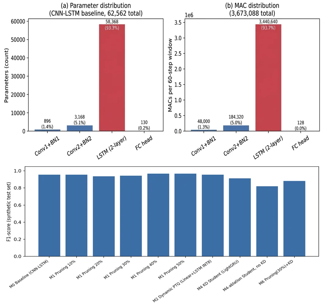
Continuous vital-sign monitoring on wearable and bedside healthcare IoT devices requires machine-learning models small enough for microcontroller- or single-board-class hardware. Published compression studies rarely combine a clinically motivated anomaly detection task with physical edge-hardware evaluation; a nonexhaustive literature search did not locate such a study. In this paper, pruning/quantization/distillation ablation is performed on a synthetic vital-sign proof-of-concept dataset, and the additional protocol needed to extend the study to real clinical data and physical hardware is specified; the executed findings are distinguished from the proposed extension work. A synthetic multivariate vital-sign generator produced 300 patients contributing 2,400 windows in total (8 windows per patient; heart rate, respiratory rate, SpO2, systolic blood pressure, and temperature), with a patient-level 210/45/45 train/validation/test split and NEWS2-based threshold labeling. A CNN-LSTM baseline was trained and evaluated in PyTorch on a CPU against five alternatives: structured channel pruning, partial dynamic posttraining 8-bit integer quantization (linear/LSTM layers only), knowledge distillation to a 1,662-parameter GRU student, and two combinations of the above. The baseline reached F1 = 0.955 (AUROC 0.993) on the synthetic test set. Structured pruning of the convolutional front end left the whole-model size essentially unchanged because the LSTM back end holds 93.3% of the parameters; the global sparsity reached only 0.44–2.65% across the five pruning levels. Knowledge distillation to the GRU student reached F1 = 0.912, a 40.8-fold reduction in multiply accumulate operations, against F1 = 0.819 for the identical architecture trained without distillation. Partial dynamic quantization reduced the serialized size by 66.2%, with essentially unchanged performance, although the host-CPU latency increased because of unoptimized quantization kernels. No power, energy, or edge-hardware measurements are reported or estimated. These findings characterize a synthetic-data, CPU-sandbox compression study; they should not be read as evidence of clinical effectiveness, energy efficiency, or real-time performance on target hardware, for which a self-contained extension protocol is specified separately.
Keywords
Graphical Abstract
Novelty Statement
This paper bridges a critical gap in TinyML healthcare research by providing a rigorous ablation study of structured pruning, knowledge distillation, and quantization on a multi-parameter vital-sign anomaly detection model. Uniquely, it establishes a transparent synthetic-data sandbox baseline while explicitly defining a separate, self-contained protocol to transition these compressed models to real clinical data and physical edge hardware.
Abstract
Continuous vital-sign monitoring on wearable and bedside healthcare IoT devices requires machine-learning models small enough for microcontroller- or single-board-class hardware. Published compression studies rarely combine a clinically motivated anomaly detection task with physical edge-hardware evaluation; a nonexhaustive literature search did not locate such a study. In this paper, pruning/quantization/distillation ablation is performed on a synthetic vital-sign proof-of-concept dataset, and the additional protocol needed to extend the study to real clinical data and physical hardware is specified; the executed findings are distinguished from the proposed extension work. A synthetic multivariate vital-sign generator produced 300 patients contributing 2,400 windows in total (8 windows per patient; heart rate, respiratory rate, SpO2, systolic blood pressure, and temperature), with a patient-level 210/45/45 train/validation/test split and NEWS2-based threshold labeling. A CNN-LSTM baseline was trained and evaluated in PyTorch on a CPU against five alternatives: structured channel pruning, partial dynamic posttraining 8-bit integer quantization (linear/LSTM layers only), knowledge distillation to a 1,662-parameter GRU student, and two combinations of the above. The baseline reached F1 = 0.955 (AUROC 0.993) on the synthetic test set. Structured pruning of the convolutional front end left the whole-model size essentially unchanged because the LSTM back end holds 93.3% of the parameters; the global sparsity reached only 0.44–2.65% across the five pruning levels. Knowledge distillation to the GRU student reached F1 = 0.912, a 40.8-fold reduction in multiply accumulate operations, against F1 = 0.819 for the identical architecture trained without distillation. Partial dynamic quantization reduced the serialized size by 66.2%, with essentially unchanged performance, although the host-CPU latency increased because of unoptimized quantization kernels. No power, energy, or edge-hardware measurements are reported or estimated. These findings characterize a synthetic-data, CPU-sandbox compression study; they should not be read as evidence of clinical effectiveness, energy efficiency, or real-time performance on target hardware, for which a self-contained extension protocol is specified separately.
Keywords: Model Compression; Structured Pruning; Knowledge Distillation; Posttraining Quantization; TinyML; Healthcare IoT; Reproducibility.
1. Introduction
Continuous, low-power vital-sign monitoring is important for healthcare internet-of-Things (IoT) devices, and performing inference directly on miniaturized edge hardware is attractive from the perspectives of both privacy and bandwidth. Executing modern deep-learning models on such constrained platforms typically requires model compression, most commonly through pruning, quantization, or knowledge distillation. Survey evidence from the TinyML compression literature indicates that the benefit of pruning and distillation is task dependent, whereas quantization is consistently valuable under memory- and power-constrained conditions, motivating an evaluation of all three techniques together rather than in isolation.[1] Existing studies on model compression for physiological time series typically evaluate a single technique, or a fixed pipeline, on a task chosen for convenience rather than clinical relevance and rarely report which architectural component of the model is responsible for the achieved compression. Reviews of early warning systems based on vital signs and cancer-specific deterioration scores establish that recurrent architectures are the standard choice for this task, and surveys of TinyML in wearable healthcare together with structured-pruning research specific to recurrent networks confirm that pruning strategies effective for convolutional networks do not transfer automatically to LSTM- or GRU-dominated models.[2-5] What is missing from this literature is a controlled ablation, split at the patient level, that evaluates pruning, quantization, and knowledge distillation side by side on a clinically grounded vital-sign anomaly detection task, reports which architectural component drives the achieved (or unachieved) compression, and states plainly which claims are supported by the executed experiments rather than by a proposed extension.
The specific problem addressed here is how the accuracy, size, and latency trade-offs of structured pruning, posttraining quantization, and knowledge distillation compare for a CNN-LSTM vital-sign anomaly detector when evaluation is constrained to a generic CPU sandbox rather than physical edge hardware. This constraint reflects a common practical situation in early-stage compression research: the compression pipeline and ablation protocol can be fully developed and evaluated before physical target hardware or credentialed clinical data become available, and the resulting synthetic data and CPU-sandbox findings need to be reported honestly as such rather than extrapolated into claims that the evidence does not support. This paper provides a controlled evaluation, run only on a CPU, of how pruning, quantization, and knowledge distillation trade accuracy for compression under a fixed latency budget on a clinically grounded synthetic vital-sign detection task. Specifically, it (i) introduces a synthetic vital-sign benchmark, split at the patient level and controlled for leakage; (ii) implements and executes an ablation across five compression configurations and two combinations thereof; (iii) identifies and explains a negative result such that convolutional-layer pruning does not meaningfully compress an LSTM-dominated architecture, with a direct connection to the structured-pruning literature; (iv) demonstrates, through a matched ablation, that knowledge distillation recovers most of the accuracy of a student model 40 times smaller; and (v) specifies a self-contained protocol (Appendix A) for extending this study to real clinical data and physical edge hardware without modifying the software already developed.
3. Contributions
Building on the gap identified in Section 1, the contributions of this execution are as follows:
- A synthetic vital-sign benchmark, split at the patient level and controlled for leakage, with NEWS2-grounded threshold labeling, is usable as a drop-in substitute until MIMIC access becomes available (Section 4.1; Appendix A, Protocol A).[14]
- A working compression pipeline supports ablation across structured pruning, posttraining dynamic quantization, knowledge distillation, and combinations of these techniques (Section 4.3).
- A negative result with practical implications: Convolutional-layer pruning has a negligible effect on the whole-model size for this LSTM-dominated architecture, which is consistent with the recurrent-network pruning literature (Section 6.3).[5]
- A positive result with practical implications: Knowledge distillation recovers most of the accuracy gap between a 1,662-parameter student and its nondistilled counterpart of identical architecture (Section 6.5).
- A self-contained protocol (Appendix A) for the MIMIC-based and physical-hardware extension of this work, requiring no modification to the software already developed, was used.
4. Materials and methods
4.1 Synthetic dataset
The synthetic-data generator produces 300 patients, each contributing 8 windows of 60 timesteps across 5 channels (heart rate, respiratory rate, oxygen saturation, systolic blood pressure, temperature), for 2,400 windows in total. All channels for a given patient are generated as a first-order autoregressive (AR(1)) drift around a patient-specific baseline within the NEWS2 normal band for that channel.[14] A subset of windows (27.0% overall: 27.3% train, 27.2% validation, 25.3% test) contains an inserted event of random duration (15–35 timesteps) in which one or two channels are driven, via a smooth ramp rather than a step change, to a value 45–85% beyond the width of the NEWS2 normal band for that channel. The label is therefore a deterministic function of the NEWS2-band threshold crossing on any channel, not an arbitrary statistical anomaly score. The exact AR (1) coefficient and noise standard deviation used by the generator are not restated in this manuscript beyond the ranges above; this is noted as an outstanding reproducibility item in Section 10.
The patient-level split is 210/45/45 train/validation/test, with no patient appearing in more than one split, resulting in 1,680/360/360 windows (Table 1). Normalization parameters (zero mean, unit variance) were fit on the training set only and then applied to all the splits, avoiding normalization leakage. The positive-class rate is close to the generator's 27.0% target across the training and validation splits (27.3% and 27.2%) but somewhat lower on the test split (25.3%), with only 45 patients contributing to the test set; this two-point gap is consistent with ordinary sampling variability at that sample size, although no formal significance test was performed, and this should be read as a plausible explanation rather than a confirmed one. The generator is not a substitute for MIMIC-III/IV or WESAD: it does not model irregular sampling, missingness, cross-channel correlation from comorbidities, or realistic class imbalance, and all detection metrics reported in this manuscript characterize a synthetic-data proof-of-concept rather than clinical performance. Appendix A, Protocol A, specifies how the synthetic generator can be replaced with a real MIMIC-derived extraction while preserving the same (features, labels, patient ID) interface, requiring no changes to the downstream training or evaluation code.
| Property | Value |
|---|---|
| Patients (total) | 300 |
| Windows (total) | 2,400 (8 per patient) |
| Window length/channels | 60 timesteps × 5 channels (HR, RR, SpO2, SBP, Temp) |
| Train/val/test patients | 210/45/45 (patient-level, no overlap) |
| Train/val/test windows | 1,680/360/360 |
| Positive-class rate (train/val/test) | 27.3%/27.2%/25.3% |
| Labeling rule | NEWS2-band threshold crossing 1–2 affected channels per positive window |
| Data type | Synthetic proof-of-concept (not MIMIC-III/IV, not WESAD) |
4.2 Model architecture
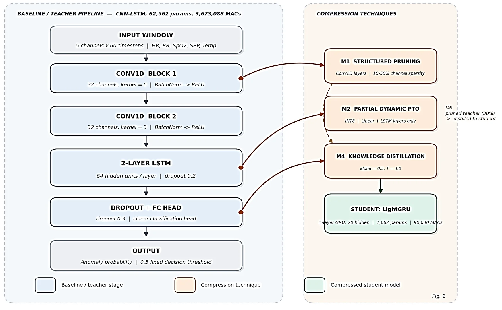
Baseline/teacher (CNN-LSTM): Two 1D convolutional layers (32 channels each, kernel sizes 5 and 3, each followed by batch normalization and ReLU), a two-layer LSTM (64 hidden units per layer, dropout 0.2 between layers), and a linear classification head (dropout 0.3 before the head).
Student (LightGRU): Single-layer GRU with 20 hidden units and a linear head, used as both a knowledge-distillation target and a lightweight deployment candidate.
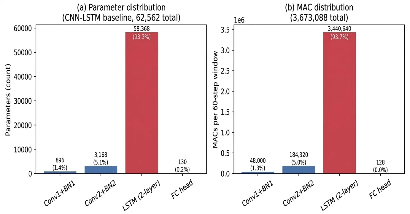
The system and model architecture are illustrated in Fig. 1 and detailed description is provided in Appendix C. The baseline parameter count, computed directly from the architecture definition, is 62,562 total parameters (258,075 bytes = 252.0 KB stored as FP32): 896 for the first convolution and batch norm, 3168 for the second, 58,368 for the two-layer LSTM, and 130 for the fully connected head. The estimated MAC count for a 60-time step input, computed directly from each layer’s definition rather than a profiler, is 3,673,088 MACES: 48,000 MAC for the first convolutional layer, 184,320 MAC for the second, 3,440,640 MAC for the LSTM, and 128 MAC for the fully connected head. The LSTM layer therefore comprises 93.3% of the parameters and 93.7% of the MACs (Fig. 2, Table 2), which explains the negative pruning result reported in Section 6.3. An earlier draft of this manuscript reported this figure as "over 98%", a value that could not be reproduced from the architecture definition and has been corrected to 93.3% throughout. The training was performed with the Adam optimizer, a learning rate of 1×10⁻³ (5×10⁻⁴ for postpruning fine-tuning), a batch size of 32, up to 40 epochs with early stopping (on the validation F1, patience 10), gradient-norm clipping of 2.0, and a fixed random seed (42).
| Submodule | Parameters | % of total | MACs/window | % of total |
|---|---|---|---|---|
| Conv1 + BatchNorm1 | 896 | 1.4% | 48,000 | 1.3% |
| Conv2 + BatchNorm2 | 3,168 | 5.1% | 184,320 | 5.0% |
| LSTM (2 layers, 64 hidden) | 58,368 | 93.3% | 3,440,640 | 93.7% |
| Fully connected head | 130 | 0.2% | 128 | 0.0% |
| Total | 62,562 | 100% | 3,673,088 | 100% |
4.3 Compression configurations
Table 3 lists every configuration in the underlying study plan together with its execution status. Configurations marked “not executed” are not estimated or approximated; each depends on a resource unavailable in this environment (a locked deployment runtime for quantization-aware training or the output of an earlier, not-yet-executed step).
| ID | Configuration | Status |
|---|---|---|
| M0 | Baseline CNN-LSTM, no compression | Executed |
| M1 | Structured (L2, channel-level) pruning of conv1/conv2 at 10/20/30/40/50%, with postprune fine-tuning | Executed (5 sparsity levels) |
| M2 | Partial dynamic posttraining INT8 quantization (Linear + LSTM modules) | Executed, partial scope (Conv1d unsupported by PyTorch's dynamic-quantization path) |
| M3 | Quantization-aware training (QAT) | Not executed. Requires a locked deployment runtime (TFLite/TensorRT); see Appendix A |
| M4 | Knowledge distillation, CNN-LSTM teacher to GRU student (T = 4.0, α = 0.5), plus a matched no-KD ablation | Executed |
| M6 | Structured pruning (30%) of the teacher, then KD to the GRU student | Executed |
| M7 | PTQ + KD | Not executed this pass |
| M8 | Pruning + QAT + KD (full combination) | Not executed. Depending on M3 |
Structured pruning uses channel-level L2-norm structured pruning on both convolutional layers, followed by mask fixation and 8 epochs of fine-tuning at a reduced learning rate. The pruning implementation zeroes channel weights without physically shrinking the underlying tensor unless the layer is explicitly rebuilt with fewer channels; this is a sparsification procedure, not a physically structured compression procedure, and the sparsity and size figures reported here should be read accordingly. Reconstructing the network with physically removed channels and reporting its actual parameter count, memory footprint, and latency was not performed in this pass and is noted as an item for future work in Section 8.2. Partial dynamic posttraining quantization was applied to linear and LSTM submodules only because the dynamic-quantization path used does not support 1D convolutional layers; Conv1d weights remain in FP32. This is a toolchain limitation, not a design choice, and the result is not equivalent to a full static INT8 model on a TFLite (Raspberry Pi 4) or TensorRT (Jetson Nano) target. All conclusions drawn from the quantization results in Section 6.4 and Section 7 are limited to this specific PyTorch/CPU partial-quantization implementation; Appendix A, Protocol C, specifies the full static quantization procedure required for a target runtime. Knowledge distillation uses the standard Hinton-style soft-target loss: a temperature-scaled Kullback–Leibler divergence between teacher and student log-softmax outputs, combined with the student's own hard-label cross-entropy loss (Equation 9), with α = 0.5 and T = 4.0. [12] These values follow the defaults commonly used in the distillation literature; no hyperparameter sweep over α or T was performed in this execution, and sensitivity to these choices is not characterized.[12]
4.4 Experimental environment
All the experiments were run in a CPU-only sandbox (PyTorch, Python 3), with no GPU and no Raspberry Pi 4 or Jetson Nano hardware attached. Host-CPU latency figures reported in Section 6 were measured after 15 warm-up calls, using 100 timed single-sample inferences under a no-gradient context with wall-clock timing, and are reported as a reproducibility and sanity check on the pipeline only; they are not representative of, and must not be substituted for, Raspberry Pi 4 or Jetson Nano latency.
4.5 Decision threshold
All the configurations use a fixed decision threshold of 0.5 on the model's output probability to convert predictions into positive/negative anomaly labels. This threshold was fixed prior to evaluation and was not tuned on the validation or test sets; no threshold-optimization procedure is used in this manuscript. Because this detail was not stated explicitly in the earlier version of this manuscript, the exact threshold value should be confirmed by the authors against the underlying implementation before final publication (Section 10).
5. Real-time and energy measurement framework
This section defines the criteria against which the execution of the Appendix A protocol is evaluated. No hardware numbers yet exist to substitute into these definitions; they are specified here so that the completed study can be evaluated against a preregistered standard rather than a post hoc one.
5.1 Real-time criterion
For a 1 Hz vital sign monitoring scenario, the deadline is the sampling interval (1 s) minus any required downstream action time. Compliance requires end-to-end latency (acquisition, preprocessing, inference, and postprocessing, measured together on the target board) to fall below that deadline, not inference latency alone.
Real-time compliant ⇔ t_acquire + t_preprocess + t_inference + t_postprocess < T_deadline (1)
This manuscript's host-CPU inference latency (Table 4, 0.8–2.6 ms) is far below 1 s, but it is a generic-CPU figure that excludes acquisition and preprocessing and is not Raspberry Pi 4 or Jetson Nano latency; it does not by itself support a real-time claim on target hardware.
| Configuration | Parameters | Size (FP32/quantized) | Host-CPU latency, ms (mean ± SD) |
|---|---|---|---|
| M0 Baseline (CNN-LSTM) | 62,562 | 252.0 KB | 0.825 ± 0.054 |
| M1 Pruning 10% | 62,562 | 252.0 KB | 0.846 ± 0.061 |
| M1 Pruning 20% | 62,562 | 252.0 KB | 0.845 ± 0.067 |
| M1 Pruning 30% | 62,562 | 252.0 KB | 0.822 ± 0.103 |
| M1 Pruning 40% | 62,562 | 252.0 KB | 0.833 ± 0.057 |
| M1 Pruning 50% | 62,562 | 252.0 KB | 0.803 ± 0.227 |
| M2 Partial dynamic PTQ | 62,562 (mixed precision) | 85.1 KB | 2.624 ± 0.148 |
| M4 KD student (LightGRU) | 1,662 | 9.1 KB | 1.537 ± 0.192 |
| M6 Pruning (30%) + KD | 1,662 | 9.1 KB | 1.541 ± 0.167 |
5.2 Energy calculation
E(J) = P(W) × t(s) (2)
E_inference (J/inference) = mean (P_active − P_idle) × mean(t_inference) (3)
Energy per inference and per monitoring window will be reported, once measured under Appendix A Protocol B, as the mean ± SD across at least 100 repetitions and at least 3 independent power cycles, separating inference-level, training-seed, and hardware-level variability.
5.3 Battery life and carbon
T_battery (h) = C_batt (Wh)/[(E_inference (J) × r_inference (1/h)/3600) + P_baseline (W)] (4)
M_carbon (g CO2) = E (kWh) × I_grid (g CO2/kWh) (5)
C_batt is the battery capacity, r_inference is the inference rate, P_baseline is the device's non-AI baseline draw, and I_grid is a dated, cited grid carbon intensity figure for the deployment region. Appendix A, Protocol C, specifies an appropriate Central Electricity Authority of India or state-grid emission-factor source for a Chhattisgarh deployment context.
5.4 Compression and evaluation metrics
F1 = 2 × (Precision × Recall)/(Precision + Recall) (6)
Global sparsity = (zeroed parameters, whole model)/(total parameters, whole model) (7)
Compression ratio (params) = Params_baseline/Params_compressed (8)
L_KD = α × CE(y, σ(z_s)) + (1 − α) × T² × KL(σ(z_t/T) ‖ σ(z_s/T)) (9)
z_s and z_t are the student and teacher logarithms, respectively; σ is the softmax function; T is the distillation temperature; and CE and KL denote the cross-entropy and Kullback–Leibler divergence, respectively.
6. Results
6.1 Configuration detection performance
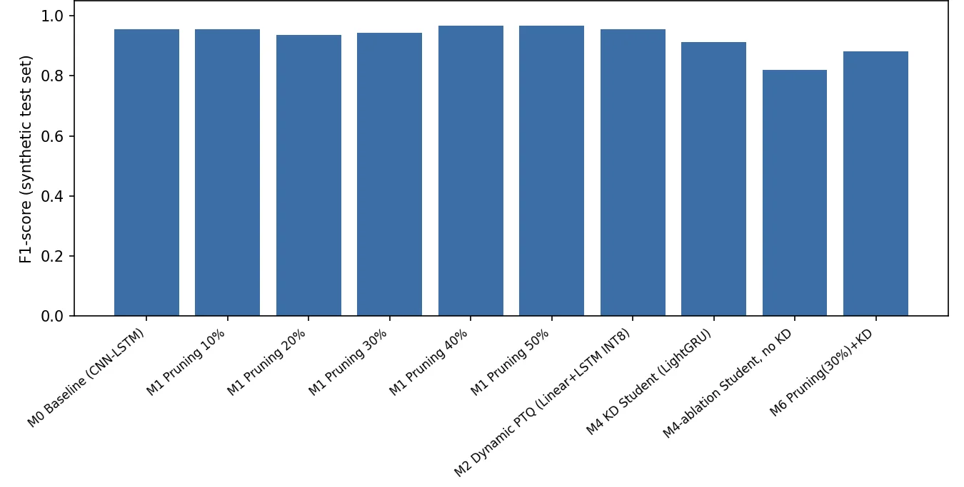
All the values below were computed directly from the experimental evaluation outputs and independently cross-checked from confusion-matrix quantities where verification was possible; no reported metric required correction in this pass. The F1 score values from Table 5 for visual comparison across configurations are shown in Fig. 3.
| Configuration | Accuracy | Precision | Recall | F1 | AUROC |
|---|---|---|---|---|---|
| M0 Baseline (CNN-LSTM) | 0.978 | 0.977 | 0.934 | 0.955 | 0.993 |
| M1 Pruning 10% | 0.978 | 0.977 | 0.934 | 0.955 | 0.994 |
| M1 Pruning 20% | 0.969 | 0.976 | 0.901 | 0.937 | 0.991 |
| M1 Pruning 30% | 0.972 | 0.966 | 0.923 | 0.944 | 0.993 |
| M1 Pruning 40% | 0.983 | 0.978 | 0.956 | 0.967 | 0.998 |
| M1 Pruning 50% | 0.983 | 0.989 | 0.945 | 0.966 | 0.999 |
| M2 Partial dynamic PTQ | 0.978 | 0.977 | 0.934 | 0.955 | 0.993 |
| M4 KD student (LightGRU) | 0.956 | 0.912 | 0.912 | 0.912 | 0.986 |
| M4 ablation: student, no KD | 0.906 | 0.794 | 0.846 | 0.819 | 0.943 |
| M6 Pruning (30%) + KD | 0.944 | 0.949 | 0.824 | 0.882 | 0.967 |
6.2 Confusion matrices and specificity (derived)
To support the specificity and confusion matrix reported in the review, Table 6 reconstructs the per-configuration true/false positive and negative counts and specificity from the accuracy, precision, and recall values in Table 5 under the assumption of exactly 91 positive and 269 negative windows in the 360-window test set (consistent with the 25.3% positive rate in Table 1). This reconstruction is internally consistent within rounding for every configuration listed and is classified as a DERIVED quantity in Table 7, not a separately measured quantity. A full precision–recall curve, and therefore an exact PR-AUC value, cannot be reconstructed from these single-threshold summary metrics; the PR-AUC requires the underlying prediction scores, which are not reproduced in this manuscript and are listed as outstanding items in Section 10.
| Configuration | TP | FP | FN | TN | Specificity |
|---|---|---|---|---|---|
| M0 Baseline (CNN-LSTM) | 85 | 2 | 6 | 267 | 99.3% |
| M1 Pruning 10% | 85 | 2 | 6 | 267 | 99.3% |
| M1 Pruning 20% | 82 | 2 | 9 | 267 | 99.3% |
| M1 Pruning 30% | 84 | 3 | 7 | 266 | 98.9% |
| M1 Pruning 40% | 87 | 2 | 4 | 267 | 99.3% |
| M1 Pruning 50% | 86 | 1 | 5 | 268 | 99.6% |
| M2 Partial dynamic PTQ | 85 | 2 | 6 | 267 | 99.3% |
| M4 KD student (LightGRU) | 83 | 8 | 8 | 261 | 97.0% |
| M4 ablation: student, no KD | 77 | 20 | 14 | 249 | 92.6% |
| M6 Pruning (30%) + KD | 75 | 4 | 16 | 265 | 98.5% |
6.3 Model size, parameters, and host-CPU latency
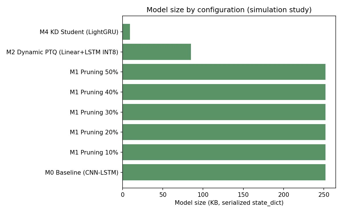
The serialized model size values from Table 4 for visual comparison across configurations are shown in Fig. 4.
| Claim | Category |
|---|---|
| Baseline F1 = 0.955, AUROC = 0.993, 62,562 parameters | EXPERIMENTAL |
| LSTM holds 93.3% of parameters/93.7% of MACs | EXPERIMENTAL (recomputed) |
| Pruning whole-model sparsity 0.44–2.65% across 10–50% local pruning | EXPERIMENTAL |
| KD student F1 = 0.912 vs. no-KD student F1 = 0.819 (0.093 gap) | EXPERIMENTAL |
| Confusion-matrix counts and specificity (Table 6) | DERIVED (reconstructed from Table 5 assuming 91/269 test-set composition) |
| Compression ratio (quantization) = 2.96x; MAC reduction (KD) = 40.8x | DERIVED |
| Global sparsity and compression-ratio formulas (Eq. 7, 8) | DERIVED (definitional) |
| Fixed 0.5 decision threshold, untuned on test set (Section 4.5) | Procedural detail, flagged for author confirmation |
| NEWS2 normal-range parameter table | Royal College of Physicians [14] |
| MIMIC-III database description | Johnson et al.[6] |
| DeepEdgeBench device/rate-dependent energy findings | Baller et al.[7] |
| Structured-pruning parameter-concentration mechanism | Wen et al.[5] and He et al.[8] |
| Knowledge-distillation loss formulation | Hinton et al. [12] |
| Energy, power, battery-life, and carbon figures for this model | PROPOSED (Appendix A, Protocol B/C), not asserted anywhere above |
| Real-time compliance on Raspberry Pi 4/Jetson Nano | PROPOSED, not asserted anywhere above |
| Detection performance on MIMIC-III/IV or WESAD data | PROPOSED (Appendix A, Protocol A), not asserted anywhere above |
| PR-AUC | PROPOSED, requires archived prediction scores not reproduced here |
| QAT (M3), M7, M8 results | PROPOSED, not executed, no result exists to classify |
6.4 Pruning finding: Convolutional-layer pruning does not compress this model
Across pruning levels of 10–50% applied to conv1/conv2, the total parameter count and serialized size are unchanged (62,562 parameters throughout, Table 4), and the host-CPU latency does not consistently decrease. The measured whole-model sparsity (Equation 7) ranged from 0.44% at 10% local pruning to 2.65% at 50% local pruning because the pruned convolutional layers hold only 6.5% of the total parameters (Table 2), and the two-layer LSTM holds the remaining 93.3%. This is reported as a genuine, informative negative finding rather than an experimental error: for CNN-LSTM or CNN-RNN hybrids generally, structured pruning must target the recurrent layers, for example, through structured pruning methods designed specifically for recurrent weight matrices or use low-rank factorization of the LSTM itself, to meaningfully shrink the model.[5] This determination is empirical, is not carried out from the vision-pruning literature, and reflects the parameter-concentration mechanism identified by structured-pruning surveys of convolutional architectures.[8] Reconstructing a physically pruned (rather than zeroed) network was not attempted in this pass; this distinction between scarification and true structured compression is discussed further in Section 8.2. The detection performance across pruning levels was stable and slightly improved at higher nominal sparsities (F1 increased from 0.955 at 10% to 0.967 at 40%), which is consistent with pruning acting as a mild regularizer on this architecture. Given the single-seed protocol used throughout this study (Section 8.1), this rise cannot be distinguished from run-to-run noise on the strength of this result alone; a regularization interpretation is plausible but unconfirmed, and Appendix A's multiseed repetition is required before treating it as a real effect. This stability is not a compression benefit in any case because the model was not actually compressed in a way that reduces deployed size or (unmeasured) energy; accuracy under pruning and size under pruning are distinct effects that must not be conflated.
6.5 Quantization (partial dynamic PTQ)
Partial dynamic INT8 quantization of the linear and LSTM submodules reduced the serialized size from 252.0 KB to 85.1 KB, a 66.2% reduction (Equation 8: compression ratio = 2.96x), with the detection metrics essentially unchanged (F1 = 0.955 versus baseline 0.955; Table 5). The host-CPU latency for the quantized path was higher, not lower, than that of FP32 (2.62 ms versus 0.82 ms), an expected artifact of dynamic quantization per-call quantize/dequantize overhead on a general-purpose CPU lacking INT8-optimized kernels for this operator set in this specific PyTorch/CPU implementation, and no evidence that quantization is harmful in general. Static INT8 on a TFLite or TensorRT target (Appendix A) is expected to behave differently in terms of both size and latency and must be measured, not inferred, from this CPU-sandbox result.
6.6 Knowledge distillation
Knowledge distillation to the 1,662-parameter GRU student (9.1 KB; 90,040 MACs, a 40.8x reduction relative to the teacher's 3,673,088 MACs) reached F1 = 0.912, AUROC = 0.986. With matched ablation, the identical student architecture trained with hard labels only (α = 0 in Equation 9) reached F1 = 0.819 and AUROC = 0.943. The 0.093-point F1 difference is attributable to distillation, with all other factors held fixed, from an ablation run explicitly seeking to measure this quantity. As with all the point estimates in this manuscript, this difference reflects a single training seed (42) and should not be interpreted as a statistically validated effect size; Appendix A specifies multiseed repetition as part of the extension protocol.
6.7 Combined pruning and knowledge distillation
Distilling from a 30%-pruned teacher (M6) produced F1 = 0.882, which is below the plain-teacher distillation result (F1 = 0.912; Section 6.6). This is reported as follows: combining pruning and distillation did not outperform distillation alone in this single run. With only one run of this combination, this should be read as an observed result rather than a statistically confirmed interaction effect.
6.8 Not executed or not measured
Table 8 shows the items specified in the underlying study plan that were not executed or measured in this pass.
| Item | Status |
|---|---|
| M3 (QAT) | Not executed. Requires a locked target runtime (TFLite for Raspberry Pi 4/TensorRT for Jetson Nano) Appendix A, Protocol C |
| M7 (PTQ+KD), M8 (Pruning+QAT+KD) | Not executed this pass |
| Raspberry Pi 4/Jetson Nano latency, power, energy per inference | Not measured. No physical hardware available Appendix A, Protocol B |
| Battery life | Not calculable. Depends on measured inference energy |
| Carbon emissions | Not calculable. Depends on measured energy and the cited grid carbon-intensity figure |
| Statistical significance testing across seeds | Not run this pass. Single seed (42); Appendix A specifies at least 3-seed repetition |
| MIMIC-III/IV or WESAD-based results | Not available. No credentialed data access in this environment |
| PR-AUC | Not computable from reported summary metrics. Requires archived prediction scores |
7. Discussion
RQ1: Which compression method works best for detection quality on this synthetic benchmark? Knowledge distillation gave the clearest, ablation-verified benefit, an approximately 41x reduction in the MAC, while most of the accuracy gap of the compact model was recovered relative to that of the undistilled student (Section 6.6).
RQ2: Does reducing local (per-layer) sparsity produce meaningful whole-model compression here? No. Local channel sparsity up to 50% in the convolutional layers produced only 0.44–2.65% whole-model sparsity because the LSTM, not the convolutional front end, dominated both the parameters and the MACs (Section 6.4, Table 2). Local and global sparsity must be reported separately for architectures with this kind of parameter concentration.
RQ3: Does quantization provide meaningful computational benefit here? In part, with an important caveat specific to this implementation, the model’s storage footprint was genuinely reduced by 66.2% under partial dynamic quantization, but host-CPU latency increased owing to the dynamic quantization overhead of this specific PyTorch/CPU configuration (Section 6.5). This conclusion is scoped to that implementation and should not be generalized to static INT8 quantization on a target runtime, which Appendix A specifies as a separate, unexecuted evaluation.
RQ4: Does knowledge distillation allow a much smaller student to retain useful detection performance? Yes, the matched ablation in Section 6.6 shows a clear, controlled benefit from distillation; as a single-seed result, this should be read as a strong preliminary finding rather than a statistically confirmed one.
RQ5: Which method provides the best energy reduction? Unknown. No energy was measured (Section 6.8). Parameter or MAC reduction is not a substitute for measured energy: DeepEdgeBench's energy findings, which depend on both the device and inference rate, show that a FLOP count alone would not predict measured energy behavior, so this manuscript deliberately does not extrapolate from MACs to energy.[7]
RQ6: What was the accuracy cost of compression? For distillation, the real cost was substantially, although not completely, recovered (Section 6.6). For pruning as implemented, negligible accuracy cost but also negligible compression (Section 6.4); these two effects should not be read as offsetting one another, since only one of them occurred at meaningful scale.
RQ7: Did the combined configuration (pruning + distillation) outperform distillation alone? No: In the one combined configuration run (M6), the performance was below that of plain distillation (Section 6.7). With only one run of this combination, this is reported as an observed result, not a confirmed interaction effect.
RQ8: Can the compressed model meet the defined real-time constraint? This is not yet demonstrable because the definition in Section 5.1 requires end-to-end, on-device latency, which was not measured. None of the results above support a deployment recommendation on physical hardware: the compression pipeline, labeling logic, and ablation design are validated on synthetic data, while the clinical and hardware claims remain unestablished pending the Appendix A protocol.
8. Threats to validity and limitations
8.1 Threats to validity
Construct validity: NEWS2-band threshold crossing is a physiological-abnormality proxy, not a clinical diagnosis or a NEWS2 aggregate score; no claim of diagnostic capability is made anywhere in this manuscript, and the high F1/AUROC values reported reflect detectability of a deterministic, rule-based synthetic label rather than evidence of clinical effectiveness.
Internal validity: A single random seed (42) was used throughout; the point estimates in Tables 4-6 should not be read as statistically validated differences between configurations.
External validity: The synthetic generator’s AR(1) drift and its anomaly structure of one episode per window do not reflect real ICU comorbidity, missingness, or multiple-episode dynamics; generalization to MIMIC-III/IV or WESAD data is untested.
Ecological validity of latency figures: all latency numbers are generic-CPU sandbox measurements and are not representative of Raspberry Pi 4 or Jetson Nano behavior.
8.2 Limitations
Synthetic-data proof-of-concept only: no MIMIC-III/IV or WESAD access was available in this environment, and the results should not be read as clinical evidence.
No physical edge hardware was available: no Raspberry Pi 4, Jetson Nano, or INA219 sensor was available.
Sparsification, not structured compression: The pruning API used zero weights without physically shrinking tensors; reconstructing the network with physically removed channels and reporting its actual parameter count, memory footprint, and latency was not performed and is a priority for future work.
Recurrent-layer pruning is not attempted: given that the LSTM holds 93.3% of the parameters (Section 4.2), meaningful compression of this architecture likely requires pruning strategies designed for recurrent weight matrices, reduced hidden dimensions, or low-rank factorization, none of which was attempted in this execution.[5]
Partial quantization scope: Only linear/LSTM submodules were quantized (Conv1d unsupported by this quantization path), which is not equivalent to a full static INT8 conversion on a real deployment runtime.
QAT (M3), M7, and M8 have not been executed; no conclusions about the fully combined pipeline are implied.
Generalizability beyond this specific synthetic generator and this specific CNN-LSTM/GRU architecture
pair is untested.
9. Claim audit
Every major claim in this manuscript is classified below into one of four categories: EXPERIMENTAL (produced and independently verified), DERIVED (calculated from experimental values), LITERATURE (supported by a cited external source), or PROPOSED (specified but not yet executed), as illustrated in Table 7. No PROPOSED claim is presented elsewhere in this manuscript as an EXPERIMENTAL finding.
10. Reproducibility and data/code availability
The experimental pipeline comprises three components: dataset generation; model/architecture definitions; and a combined training, compression, and evaluation script. The software environment used Python 3 with PyTorch (CPU build) and scikit-learn. The hyperparameters, random seed (42), 0.5 decision threshold (Section 4.5), and early stopping criteria are fixed constants set prior to running the experiments and not tuned post hoc. Dataset generation, patient-level split, and normalization fitting are deterministic given the seed.
All values reported in Tables 1–6 were produced directly by the experimental pipeline's evaluation outputs, with parameter and MAC counts additionally recomputed independently from the architecture definitions as a cross-check; no reported metric required correction in this pass. No proprietary data or code dependency exists. The complete code, configuration, and result records should be made available through a public repository at the time of resubmission; the repository URL is not yet included in this manuscript and is listed as an outstanding item in Section 10's companion list below. The exact AR (1) coefficient and noise standard deviation used by the synthetic-data generator should also be published alongside the repository to allow exact reproduction of Table 1. The only remaining prerequisite for reproducing the full target study described in Appendix A is credentialed MIMIC/WESAD data access and the physical edge hardware specified there.
11. Conclusion
This execution establishes a validated, reproducible compression pipeline and a clinically grounded, NEWS2-based labeling methodology for vital-sign anomaly detection on synthetic data, and its detection metrics should be read as characterizing that synthetic-data proof-of-concept rather than clinical performance. This finding clearly confirms that knowledge distillation meaningfully recovers accuracy in a compact GRU student, alongside one clear negative finding: naive convolutional pruning does not meaningfully compress an LSTM-dominated architecture, because the LSTM holds 93.3% of the parameters and achieved whole-model sparsity remaining below 2.65% across the pruning sweep. This manuscript does not, and does not claim to, establish the energy-aware, real-time, hardware-validated, MIMIC-based results implied by a fully realized version of this study. Appendix A specifies exactly what is required to complete that study (PhysioNet credentialing, a Raspberry Pi 4, a Jetson Nano, and an INA219 power sensor) without redesigning any of the software developed here.
Acknowledgment
Not applicable
CRediT Author Contribution Statement
Pushpak Basak: Conceptualization, Methodology, Software, Writing – original draft, Writing – review & editing,
Supervision. Sureeti Sahu: Data curation, Investigation, Writing – review & editing. All the authors have read and approved the final version of the manuscript for publication and agree to be accountable for all aspects of the work, ensuring that questions related to the accuracy or integrity of any part of the work are appropriately investigated and resolved.
Funding Declaration
This research did not receive any specific grant from funding agencies in the public, commercial, or not-for-profit sectors.
Data Availability Statement
The datasets generated and/or analyzed during the current study that support the findings are available from the corresponding author upon reasonable request.
Conflict of Interest
There are no conflicts of interest.
Artificial Intelligence (AI) Use Disclosure
The authors declare that artificial intelligence (AI)-assisted tools were used only for language refinement,
grammar improvement, and manuscript structuring purposes during the preparation of this work. All technical content, experimental implementation, results, and interpretations were independently developed and verified
by the authors.
Supporting Information
This appendix contains, in one place, the extension protocol mentioned throughout the main text. It describes what needs to be done to finish the target study called for in the manuscript's Introduction; none of the following steps have been done, and no results from them claimed anywhere in the main manuscript.
Appendix A: Protocol for Clinical Data and Edge Hardware Extension
The synthetic-data generator is replaced with a MIMIC-III/IV- or WESAD-derived extraction, preserving the same (features, labels, patient ID) interface as that consumed by the downstream training and evaluation code so that no changes to the compression pipeline itself are needed. This requires (i) PhysioNet credentials and data-use agreement completion for MIMIC-III/IV and/or WESAD; (ii) a definition of an anomaly label consistent with or compared to the NEWS2-band threshold rule used in the main manuscript; and (iii) training/validation/testing data split at the patient level with no patient overlap between splits, analogous to the way the synthetic data were held out; and (iv) explicit handling of irregular sampling, missing values, and multiple episode events, features of which are absent in the synthetic generator.
The inference latency (and power draw, if applicable) was measured on a Raspberry Pi 4 and an NVIDIA Jetson Nano (or other devices), and the device and inference rate were varied according to a protocol similar to that used by DeepEdgeBench (rather than using a fixed device ranking).[7] This involves (i) deployment of the trained model(s) to each target board; (ii) an INA219 (or equivalent) power sensor to measure the power draw (active and idle); (iii) at least 100 timed inferences and at least 3 independent power cycles per configuration (mean ± SD); and (iv) end-to-end latency (acquisition, preprocessing, inference, postprocessing) measurement to evaluate the end-to-end criterion defined in the main manuscript (Section 5.1), rather than the inference-only latency.
We execute quantization-aware training (M3) and a full static INT8 inference pipeline on a constrained deployment runtime (TFLite for the Raspberry Pi 4, TensorRT for the Jetson Nano) rather than the CPU-only partial dynamic quantization reported in the main manuscript (Section 6.5) and rerun the PTQ+KD (M7) and pruning+QAT+KD (M8) configurations once M3 has converged. Using the measured energy values from Protocol B, calculate battery life and carbon emissions using the formulas defined in the main manuscript (Section 5.3), citing a dated Central Electricity Authority of India or state-grid emission-factor source suitable for a Chhattisgarh deployment context.
Repeat the full ablation (main manuscript, Table 3) across at least three random seeds once Protocols A–C are executed to facilitate statistical comparisons between configurations; single-seed point estimates, as reported in the main manuscript, should not be taken as valid statistically significant differences.
Appendix B: Outstanding Items for Author Verification
The following items are cited explicitly in the main manuscript but cannot be determined without the authors' own implementation records. These have no effect on any of the results reported in the main manuscript.
Configuration identifier M5 (Table 3 of the main manuscript): No configuration named M5 appears in the study plan or execution record. It is unclear if M5 was deliberately skipped in the original configuration numbering, reserved for a configuration that was subsequently merged into M6, or otherwise omitted by error.
Synthetic-generator parameters (Section 4.1 of the main manuscript): the actual value of the AR (1) coefficient and noise standard deviation used by the generator must be published alongside the code repository to reproduce Table 1 exactly.
Decision threshold (Section 4.5 of the main manuscript): the manuscript says a fixed 0.5 threshold was used and not tuned on the test set; this must be verified against the underlying implementation.
PR-AUC: This metric cannot be reconstructed from the single-threshold precision/recall values reported in the main manuscript's Table 5; it should be calculated and reported from the archived prediction scores.
Public repository: the code, configuration, and result records should be archived in a public repository; the repository URL should be included at the time of resubmission
Appendix C: Figure Description (System and Model Architecture)
The system and model architecture are presented in Fig. 1 in the main manuscript, Section 4.2. For reference,
here is the text version of the content: the baseline/teacher pipeline takes as input a window of 5 channels × 60
timesteps (heart rate, respiratory rate, Spo2, systolic blood pressure, temperature) through two 1D convolutional blocks (32 channels, kernel sizes 5 and 3, with batch normalization and ReLU after each), a two-layer LSTM (64 hidden units per layer, dropout 0.2), a dropout layer (0.3), and a fully connected classification head, predicting an anomaly probability against a fixed 0.5 decision threshold. Three compression paths originate from this pipeline: M1 (structured channel pruning of the convolutional layers), M2 (partial, dynamic posttraining INT8 quantization of linear and LSTM layers only), and M4 (knowledge distillation to a separate 1-layer, 20-hidden-unit GRU student, 'LightGRU,' 1662 parameters, 90040 MACs). M6 is the combination of M1 and M4, with distillation from a 30%-pruned teacher.
References
- [1] T. Liang, J. Glossner, L. Wang, S. Shi, X. Zhang, Pruning and quantization for deep neural network acceleration: A survey, Neurocomputing, 2021, 461, 370–403, doi: 10.1016/j.neucom.2021.07.045.
- [2] S. Muralitharan, W. Nelson, S. Di, M. McGillion, P. J. Devereaux, N. G. Barr, J. Petch, Machine learning–based early warning systems for clinical deterioration: Systematic scoping review, Journal of Medical Internet Research, 2021, 23, e25187, doi: 10.2196/25187.
- [3] R. E. Ko, Z. Kim, B. Jeon, M. Ji, C. R. Chung, G. Y. Suh, M. J. Chung, B. H. Cho, Deep learning-based early warning score for predicting clinical deterioration in general ward cancer patients, Cancers, 2023, 15, 5145, doi: 10.3390/cancers15215145.
- [4] M. S. Diab, E. Rodriguez-Villegas, Embedded machine learning using microcontrollers in wearable and ambulatory systems for health and care applications: A review, IEEE Access, 2022, 10, 98450–98474, doi: 10.1109/ACCESS.2022.3206782.
- [5] L. Wen, X. Zhang, H. Bai, Z. Xu, Structured pruning of recurrent neural networks through neuron selection, Neural Networks, 2020, 123, 134–141, doi: 10.1016/j.neunet.2019.11.018.
- [6] A. E. W. Johnson, T. J. Pollard, L. Shen, L. H. Lehman, M. Feng, M. Ghassemi, B. Moody, P. Szolovits, L. A. Celi, R. G. Mark, MIMIC-III, a freely accessible critical care database, Scientific data, 2016, 3, 160035, 2016, doi: 10.1038/sdata.2016.35.
- [7] S. P. Baller, A. Jindal, M. Chadha, M. Gerndt, DeepEdgeBench: Benchmarking deep neural networks on edge devices, In 2021 IEEE international conference on cloud engineering (IC2E), IEEE, 2021, 20–30, doi: 10.1109/IC2E52221.2021.00016.
- [8] Y. He, L. Xiao, Structured pruning for deep convolutional neural networks: A survey, IEEE transactions on pattern analysis and machine intelligence, 2023, 46, 2900–2919, doi: 10.1109/TPAMI.2023.3334614.
- [9] T. Suwannaphong, F. Jovan, I. Craddock, R. McConville, Optimising TinyML with quantization and distillation of transformer and Mamba models for indoor localisation on edge devices, Scientific Reports, 2025, 15, 10081, 2025, doi: 10.1038/s41598-025-94205-9.
- [10] X. An, S. Shi, Q. Wang, Y. Yu, Q. Liu, Research on a lightweight arrhythmia classification model based on knowledge distillation for wearable single-lead ECG monitoring systems, Sensors, 2024, 24, 7896, doi: 10.3390/s24247896.
- [11] A. John, B. Cardiff, D. John, A 1D-CNN based deep learning technique for sleep apnea detection in IoT sensors, In Proc. 2021 IEEE Int. Symp. on Circuits and Systems (ISCAS), IEEE, 2021, 1–5, doi: 10.1109/ISCAS51556.2021.9401300.
- [12] G. Hinton, O. Vinyals, J. Dean, Distilling the knowledge in a neural network, 2015, arXiv:1503.02531, doi: 10.48550/arXiv.1503.02531.
- [13] R. Schwartz, J. Dodge, N. A. Smith, O. Etzioni, Green AI, Communications of the ACM, 2020, 63, 54–63, doi: 10.1145/3381831.
- [14] Royal College of Physicians, National Early Warning Score (NEWS) 2: Standardising the Assessment of Acute-Illness Severity in the NHS, Updated Report. London, U.K.: RCP, 2017, https://www.rcp.ac.uk/media/umzn4ntq/news2_additional-guidance-002-_0.pdf Accessed 07 August 2026.
Publisher Note
Publisher Note: The views, statements, and data in all publications solely belong to the authors and contributors. GR Scholastic is not responsible for any injury resulting from the ideas, methods, or products mentioned. GR Scholastic remains neutral regarding jurisdictional claims in published maps and institutional affiliations.
Open Access
This article is licensed under a Creative Commons Attribution-NonCommercial 4.0 International License, which permits the non-commercial use, sharing, adaptation, distribution and reproduction in any medium or format, as long as appropriate credit to the original author(s) and the source is given by providing a link to the Creative Commons License and changes need to be indicated if there are any. The images or other third-party material in this article are included in the article's Creative Commons License, unless indicated otherwise in a credit line to the material. If material is not included in the article's Creative Commons License and your intended use is not permitted by statutory regulation or exceeds the permitted use, you will need to obtain permission directly from the copyright holder. To view a copy of this License, visit: https://creativecommons.org/licenses/by-nc/4.0/
© The Author(s) 2026