

 Open Access||Research Article
A Hidden Markov Framework for Concept Drift Detection and Classification
Kailas Kunjumon1, Aksa Maria Paul1, Mariya K Joby1, Hemanth KS1, Bitan Misra2
1 Christ University, Bangalore, Karnataka, 560029, India
2 Department of Computer Science and Engineering, Techno International New Town, Kolkata, 700156, India
Abstract
Machine learning systems deployed in real-world environments frequently encounter non-stationary data streams in which the underlying data-generating distribution shifts over time. This phenomenon, known as concept drift, causes progressive model degradation if left undetected. Existing detection methods largely treat drift as a binary event, ignoring the temporal dynamics and structural diversity of distributional change. In this paper, we present the Hidden Markov Model (HMM)-based drift tracking (HDT) system, a framework that models concept drift as a latent probabilistic process over three hidden states, i.e., stable, warning, and drift using an HMM. The Viterbi algorithm is employed to decode the most probable state sequence from a multivariate observation vector constructed from sliding-window statistical features of the data stream, including the sample mean, variance, Kolmogorov-Smirnov (KS) statistic, and model error rate. Upon detecting a drift event, HDT classifies it into one of two primary structural categories as sudden drift and gradual drift and further determines whether each event is harmful or benign based on a feature-derived severity criterion. Experiments conducted on the university of California (UCI) gas sensor array drift dataset, comprising 13,810 post-initialization observations across ten sensor batches collected over 36 months, demonstrate the system's ability to track drift onset, progression, and recovery in a physically motivated non-stationary stream. Results shows 2,575 confirmed drift events, with 1,021 classified as harmful and 1,554 as non-harmful. The HDT system offers a principled and interpretable alternative to threshold-based detectors for monitoring deployed machine learning systems in dynamic environments.
Keywords
Graphical Abstract
Novelty Statement
This work introduces a Hidden Markov Model (HMM)-based Drift Tracking (HDT) framework that formulates concept drift detection as a probabilistic latent-state inference problem instead of conventional threshold-based binary decisions.
1. Introduction
Many machine learning models operate on the premise that the training and inference distributions are the same. However, this premise fails frequently. Time-varying properties arise for data sources including physical sensors, stock market data, user interaction histories, and medical monitoring systems. If the distribution P(X, Y) undergoes an evolution between training and deployment, called concept drift, the model suffers in performance according to the degree of change in the distribution.[1-3] Traditional drift detection methods tackle this challenge using threshold-based techniques based on summarizations of the stream under observation. For instance, the drift detection method keeps track of error rates and sounds the alarm once the error rate crosses a certain multiple of the minimum value ever recorded.[4] Similarly, adaptive windowing (ADWIN) keeps track of a resizable window and alarms when there is a large enough difference between the means of the two halves of the window.[5] The Kolmogorov-Smirnov Windowing (KSWIN) method employs a non-parametric distribution test on unlabeled streams to detect drifts.[6] Even though all three algorithms provide dependable drift detections at a point in time, they suffer from a common weakness: they treat drift detection as a sequence of classification decisions.[7,8]
The limitations of binary drift detection become evident once the wide variety of drift situations that can occur in real-world scenarios are taken into account. The gradual deterioration of a gas sensor over time is inherently different from an instantaneous drift caused by contamination of the sensor through chemical exposure. A machine learning (ML) model that is applied to user data that undergoes drastic shifts due to a new platform policy would face a very different situation than an ML model operating on user data showing a slow seasonal behavioural change. The binary drift detector fails to capture the variety, offering only an indication of whether the drift happened or not. This information comes at an operational cost, as it does not allow distinguishing between types of drifts, which means the model might have to be replaced immediately in the case of an abrupt drift or incrementally adjusted in case of a slow drift, for example.
This study presents a hidden Markov model (HMM)-based drift tracking (HDT) system, where the problem of drift detection is recast in terms of probabilistic latent-state inference. Instead of imposing a threshold on the value of a univariate statistic, the HDT approach considers an HMM whose states are stable, warning, and drift. The decoding of the most likely state trajectory from the given observation sequence is done via the Viterbi algorithm. Such an architecture confers three abilities to the system, which are not available in current solutions. First, it takes into account the dynamic nature of drift by encoding the state transition through a sequence of states and not as a sequence of binary judgments. Second, the concept of early warning appears naturally in the model because warning becomes a first-order concept rather than a supplementary heuristic device. Third, post-hoc characterization of drift becomes possible because once a drift-state sequence is detected, the sequence of the observation feature values in that period could be employed for classifying the drift as either sudden or gradual and evaluating its harmfulness. The objectives of this study are as follows:
I. Develop an HMM based framework to model the drift lifecycle as a sequence of hidden latent states over a non-stationary data stream.
II. Implement the Viterbi algorithm to achieve globally consistent decoding of the most probable hidden state trajectory from multivariate feature observation sequences.
III. Classify detected drift events into structural categories such as sudden drift and gradual drift using the temporal signature of each event.
IV. Introduce and apply a harmfulness criterion to distinguish operationally critical drift events from benign distributional fluctuations.
V. Validate the HDT framework using the University of California (UCI) gas sensor array drift dataset to demonstrate its effectiveness in tracking real-world, multi-batch sensor degradation.
The organization of the paper is: in section 2, a literature review is discussed. The methodology is discussed in section 3, followed by the results explained in section 4 and the discussion in section 5. Finally, in section 6, the conclusions are reported.
2. Literature Review
Concept drift becomes an issue in stream data due to the possibility that the statistical behaviour of incoming data can be altered, affecting the predictive accuracy of the models used. Gama et al. have provided a comprehensive review on concept drift and adaptation techniques, which highlights the different types of drifts, drift detection, and adaptation.[2] Žliobaitė et al. extend this discussion by presenting real-world applications of concept drift, showing that drift occurs in domains such as sensor networks, finance, medicine, and user-behaviour analysis.[3] This supports the need for drift-aware systems in practical streaming environments. Baena-García et al. introduced the early drift detection method (EDDM), which focuses on identifying drift at an early stage by monitoring changes in prediction errors.[4] This method is useful for warning-level detection before full drift occurs. Kolter and Maloof proposed dynamic weighted majority, an ensemble-based method for handling drifting concepts.[9] Their approach dynamically changes classifier weights and adds or removes models based on performance, making it effective for adaptive learning.
Wang et al. applied a hidden Markov model with transfer learning for cooperative anomaly detection in virtualized network slicing.[10] This study shows that HMMs can model hidden system states and detect abnormal behavioural changes over time. Greco et al. proposed an unsupervised concept drift detection method using deep learning representations in real time.[11] Their work is important because it reduces dependence on labeled data, which is often unavailable in streaming environments. Losing et al. reviewed incremental online learning algorithms and compared state-of-the-art approaches.[12] Their study highlights the importance of models that can continuously update without retraining from scratch. Komorniczak and Ksieniewicz proposed unsupervised concept drift detection based on neural network activations.[13] Their method demonstrates how internal model behaviour can be used to detect distribution changes without requiring class labels. Koch et al. studied distribution shift detection for postmarket surveillance of medical artificial intelligence (AI) systems.[14] Their work emphasizes the importance of detecting shifts after deployment, especially in safety-critical applications. Xiong et al. proposed a semi-supervised comparative learning compensation method for chemical gas sensor drift.[15] This is directly relevant to gas sensor drift problems, showing that sensor data distributions can change over time and require compensation techniques.
Existing studies provide strong foundations for concept drift detection, online learning, ensemble adaptation, and sensor drift compensation (see Table 1). However, many methods either depend on labeled data[4], use ensemble-based adaptation rather than explicit hidden-state modeling[9], or focus mainly on deep representation learning.[11,13] In gas sensor drift studies, compensation methods are often proposed, but drift-state identification as stable, warning, and drift is less explicitly modeled.[15] Therefore, the research gap is the need for an unsupervised, real-time drift detection framework that combines statistical window features such as mean, variance, and KS distance with a hidden Markov model to identify hidden drift states. The proposed HDT approach addresses this gap by using HMM-based temporal state modeling, allowing the system to detect gradual changes, issue early warnings, and confirm drift in streaming gas sensor data.
Table 1: Comparative analysis of existing concept drift and adaptive learning approaches.
| Ref. | Study | Method/Approach | Strengths | Limitations | Research gap addressed by HDT |
|---|---|---|---|---|---|
| [3] | Žliobaitė et al. (2015) | Review of real-world concept drift applications | Demonstrates practical relevance across domains | Focuses on applications rather than detection methodology | No mechanism for drift-state inference or severity assessment |
| [4] | Baena-García et al. (2006) | Early Drift Detection Method (EDDM) | Provides early drift warnings using prediction errors | Requires labeled data and threshold tuning; binary decision output | No latent-state representation or drift-type classification |
| [9] | Kolter & Maloof (2007) | Dynamic Weighted Majority (DWM) | Adaptive ensemble learning under drift | Focuses on adaptation rather than explicit drift-state detection | Does not model warning, drift progression, or harmfulness |
| [10] | Wang et al. (2019) | Transfer Learning-based HMM for anomaly detection | Demonstrates effectiveness of HMMs in modeling hidden system states | Designed for anomaly detection rather than concept drift tracking | No drift-state lifecycle modeling or drift categorization |
| [11] | Greco et al. (2025) | Deep-learning representation-based unsupervised drift detection | Operates without labeled data and supports real-time detection | Limited interpretability of detected drift events | No explicit temporal state transitions or severity analysis |
| [13] | Komorniczak & Ksieniewicz (2024) | Neural activation-based unsupervised drift detection | Label-free drift monitoring | Dependent on neural network architecture and internal activations | No probabilistic state modeling or drift-type characterization |
| [14] | Koch et al. (2024) | Distribution shift detection for medical AI surveillance | Addresses deployment-stage monitoring in safety-critical systems | Detects shifts but does not characterize their progression | No latent-state inference or harmfulness evaluation |
| [15] | Xiong et al. (2024) | Semi-supervised gas sensor drift compensation | Specifically addresses sensor drift degradation | Focuses on compensation rather than drift-state identification | No warning-state modeling or drift classification |
| Proposed HDT | This Study | HMM-based Drift Tracking using Stable–Warning–Drift states and Viterbi decoding | Probabilistic temporal modeling, early warning capability, drift-type classification, harmfulness assessment, interpretable state trajectories, and unsupervised operation | Current implementation uses scalar feature aggregation and Gaussian emissions | Addresses temporal drift evolution, warning-state inference, drift categorization, and severity-aware decision support within a unified framework |
3. Methodology
3.1 Sliding-window statistical features
At each moment in time t, the most recent w points in the stream are used for the analysis; this is called a sliding window Wt. Additionally, there is a reference window Wref, which represents the first w points obtained when the stream begins. The difference between the sliding window and the reference window allows estimating the change in the data. To characterize the data, there are four statistics calculated for each of the windows:
In eq. (1), Ot is the observation vector at time step t. This is the input to the HMM every time and contains everything that the model needs in order to determine the state of the stream. μt is the sample mean of the current window Wt. This captures if the average value of the data has drifted significantly from where it was in the beginning. When there is any shift in the average level of the values, this is normally the very first indicator that something has happened to the distribution of the data. σt2 is the sample variance of the current window Wt. Variance tells us how scattered the data values are. In cases when a drift is noticeable only in the scattering of the values, but not in their average level, then this is the feature to catch such drifts. KSt is the Kolmogorov-Smirnov statistic between the current window Wt and the reference window Wref. The KS-statistic does not focus on summary statistics such as mean and variance; rather, it captures the whole picture. This is the most sensitive feature of all the above. et is the error rate of the model currently in production for the current window Wt. This is the most straightforward way to determine the impact: if the model is making more mistakes compared to its usual performance, this is indicative of the data the model was trained on being outdated relative to the new data. Together, these four numbers give a fairly complete picture of whether something has changed in the data. The KS statistic is defined as shown in eq. (2):
In eq. (2), Wt is the latest sliding window made up of the last w samples of the streaming data. Wref is the reference window sampled at the beginning of the streaming data window, capturing the baseline stable distribution. FWt(x) is the empirical cumulative distribution function (ECDF) of the window Wt. Given a particular x value, this gives the proportion of the data points in Wt that are below or equal to x — an increasing line segment starting from 0 to 1. FWref(x) is the ECDF for the reference window Wref calculated in the same manner. supx is the supremum (the maximum value across all values of x). | . | is the absolute value, since all we care about is the magnitude of the difference. In plain terms, this measures the largest gap between the distribution of values in the current window and the reference window. A small KS value means the data looks similar to when we started; a large value means something has shifted.
3.2 Formulation of the HMM
The formulation of the model is based on the use of an HMM, Λ = (A, B, π), where the state of the stream under consideration is modeled. We assume that for any instant of time t the data stream is in one of three different states which can only be inferred from observable data and are thus referred to as hidden states. There are three possible states of a data stream: stable state (S1), warning state (S2), and drift state (S3). The data in the stream is said to be stable when it matches the reference data. The warning state refers to a situation in which something changes but it is not yet considered a drift. The drift state means that there were some changes in the data in comparison to the reference data.
Transition matrix: The transition matrix A shows the probability of switching from one state to another. The elements of this matrix are computed by the Baum-Welch algorithm[16] as follows:
In eq. (3), the transition matrix row 1 is the stable state: there is an 85% possibility of continued existence of the stable state, a 12% possibility of moving to the warning state, and a 3% possibility of drifting without reaching the warning state. Row 2 is the warning state, giving the possibilities of returning to the stable state with 20%, remaining at the warning state with 65%, and drifting with 15%. Warning states have sticky data, which means that data gets stuck for some time in a limbo state and finally either becomes stable or drifts. Row 3 is the drift state: there is a 40% possibility of returning from drift state to stable state after training/recovery, a 30% possibility of remaining in the warning state, and a 30% possibility of continuing to drift. Each row sums to 1.
Emission model: each of the states produces observations with a bit of difference. This is modeled as follows:
In eq. (4), P(Ot | St = Si) is the emission probability — the probability of observing Ot assuming that at time t the underlying hidden state is Si. High values indicate that observation Ot matches state Si well, while low values indicate a bad match. N(x; μi, Σi) is a multivariate Gaussian distribution with mean vector μi and covariance matrix Σi. μi is the mean vector associated with the observed data in state Si. If stable is the hidden state, then μ1 will have a small KS value and error rate; when drift is the hidden state, μ3 will have a large KS value and error rate. Σi is the covariance matrix for state Si, describing dependencies between the four observed features in state Si — for example, in the drift hidden state, KS and error rates show correlation. In other words, each state has its own mean vector of feature values (μi) and covariance matrix (Σi). The stable state is characterized by low KS statistics and a small amount of errors; the drift state has high KS statistics and relatively high errors. The initial distribution π = [0.90, 0.08, 0.02], reflecting the prior assumption that the stream is highly likely to be stable initially.
3.3 Viterbi algorithm for state decoding
Given the HMM parameters, we now proceed to estimating the hidden states of the stream at each time instant t. The Viterbi algorithm[17] is used for this purpose. Instead of analyzing each instant t separately, the algorithm takes into account the entire history of observations up until time t and computes the most probable state sequence:
In eq. (5), S* is the most likely hidden state sequence across the whole stream — the ultimate result obtained after applying the decoding algorithm, showing whether the stream has been stable, warning, or drifting at every time step. argmaxS selects, among all possible state sequences within T time periods, the sequence with the maximum probability given the observations. P(S1, …, ST | O, Λ) is the joint probability of the state sequence conditional on observations O and model parameters Λ = (A, B, π), combining the emission probabilities (fit of each state to the observation) and the transition probabilities between states. The algorithm works efficiently through time step by step, keeping track of the best path to each state at each step:
In eq. (6), δt(i) is the probability of the most likely sequence of observations up to time t that ends in state Si at time t, calculated for every state i and every time step t. δt−1(j) is the probability of the best path at the previous time step that ends in state Sj, carried over to develop the sequence of states. aij is the probability of transitioning from state Sj to state Si, derived from the transition matrix A. maxj [ δt−1(j) · aij ] evaluates all possible prior states j and selects the one maximizing the product of probabilities — the core dynamic-programming step that avoids revisiting earlier choices. bi(Ot) is the emission probability for the current observation Ot under state i, taken from emission model B. Here i, j index the hidden states (i=1 stable, i=2 warning, i=3 drift), T is the total number of time steps, and N=3 is the number of hidden states in HDT. The algorithm runs in O(N²T) time, which is highly efficient even for extremely long data streams, and it provides the whole history of states the stream passed through while changing from stable to warning to drift.
3.4 Drift types and harmfulness
When S* is generated, every confirmed drift segment is sorted based on its type, which may be one of two: sudden drift or gradual drift. Sudden drift occurs in a sudden, rapid fashion without a long warning phase prior to the change — a steep increase in the KS statistic takes place, and this type is hard to handle since the model does not have enough time to respond before poor performance becomes apparent. Gradual drift takes time, often preceded by an extended warning phase, allowing time for adaptation; it is considered less harmful than sudden drift if warnings are addressed promptly. To evaluate whether a particular drift event was harmful enough to prompt action, we calculate the harmfulness score:
In eq. (7), H(e) is the harmfulness index associated with drift event e, on the range [0, 10]. A value of 5.0 or higher indicates that the event is harmful and the model needs retraining; below 5.0, the event can be considered benign, meaning no immediate action is needed. e is a single drift event — a contiguous sequence of time steps in the drift state found in the decoded series S*. μKS(e) is the mean KS statistic across all time steps of event e, the most significant factor impacting the score: a high mean KS statistic implies a severe deviation between current and reference data, and this component is multiplied by 5 to receive the highest weight in the final score. 1[|e|>10] adds 1 to the score if the duration of the drift event exceeds 10 time steps, since prolonged drift events usually represent a true long-term shift rather than a transient phenomenon. 1[wpre(e)<3] adds 1 to the score if fewer than 3 time steps of warning state occurred just prior to the drift event, implying a dangerously quick onset. min(10, .) caps the value at 10 regardless of the magnitude of each component.
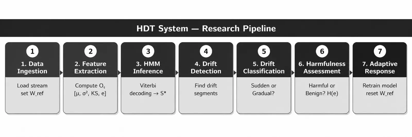
The HDT system works as a step-by-step pipeline, where each stage feeds into the next, as shown in Fig. 1. In the data ingestion stage, the raw stream data is loaded, and the first w observations are used to set up the reference window Wref. During feature extraction, at each time step, the four-feature observation vector Ot is computed from the current sliding window. In the HMM inference stage, the observation sequence is passed into the HMM, and the Viterbi algorithm decodes the most likely state sequence S*. In drift detection, the decoded sequence is scanned for stretches of consecutive drift-state time steps, and each such stretch is marked as a drift event. During drift classification, each drift event is analyzed by checking how long the warning phase lasted before it and how quickly the KS statistic rose, labeling the event as sudden or gradual. In the harmfulness assessment stage, H(e) is computed for each event to determine whether it is harmful or benign. Finally, in the adaptive response stage, harmful events trigger replacement of the live model with a newly retrained one, and the reference window is reset.

Fig. 1: Structural workflow of the HDT system.
4. Results
4.1 Dataset description
The HDT algorithm was tested on the UCI gas sensor array drift dataset.[18] The dataset was collected over about three years by means of a gas sensor array including 16 sensors exposed to six different gases across ten experiments. This dataset is popular for studying drift phenomena partly because the drift occurring in it is real and physical — sensors degrade physically as the chemicals deteriorate with time, so the drifts are not artificially induced.
Each point from the dataset contains 128 attributes, one for every possible value of each sensor. To simplify the calculations, only one point was considered for every time step by averaging all sensors' values, giving 13,910 points, of which 100 points were needed for initializing the algorithm; the remaining 13,810 points were available for conducting the experiment. The size of the window used during the feature-calculation process was set equal to 100.
4.2 Simulation results
Table 2 presents the number of time steps per each state during the entire evaluation process. Approximately 37%, 44%, and 19% of time steps were spent in the stable, warning, and confirmed drift states, respectively. The largest share going to the warning state means that the system managed to detect the onset of changes before moving to the final stage of detecting drifts — precisely what the system was expected to do. Table 3 illustrates the statistics on the confirmed drifts depending on their type and harmfulness. There were 2,575 time steps in which the system detected drifts; out of 1,861 gradual and 714 sudden drifts, gradual drifts prevail, which is natural for a dataset that features sensor degradation rather than failure. Almost half (40%) of the confirmed drifts are harmful while 60% are harmless (benign).
Table 2: Time steps distribution across the three states.
| State | Count |
|---|---|
| Stable | 5,129 |
| Warning | 6,106 |
| Drift (Confirmed) | 2,575 |
| Total | 13,810 |
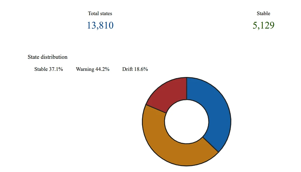
Fig. 2: Donut chart showing the proportion of time steps in each HMM state across the full evaluation stream.
Fig. 2 shows the state distribution as a donut chart. The largest pie portion is the warning state (44.2%), followed by stable (37.1%), and drift (18.6%). The predominance of the warning state means there was enough room for preparation before the official drift happened. Fig. 3 shows the comparison between the frequency of sudden drifts (714) and gradual drifts (1,861); gradual drifts happen significantly more often than sudden ones, a natural outcome for a sensor data collection in which sensors gradually become less sensitive and their readings change slowly, month after month.
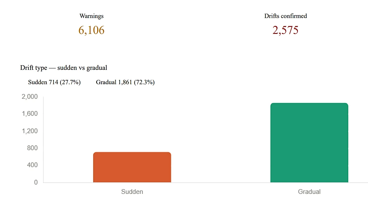
Fig. 3: Bar chart comparing the count of sudden drift events (714) and gradual drift events (1,861).
Table 3: Drift types and harmfulness levels from the gas sensor experiment.
| Drift type | Confirmed events | Harmfulness |
|---|---|---|
| Sudden drift | 714 | High — needs immediate retraining |
| Gradual drift | 1,861 | Moderate — can be managed gradually |
| Total harmful | 1,021 | Model replacement required |
| Total benign | 1,554 | Safe — no urgent action needed |
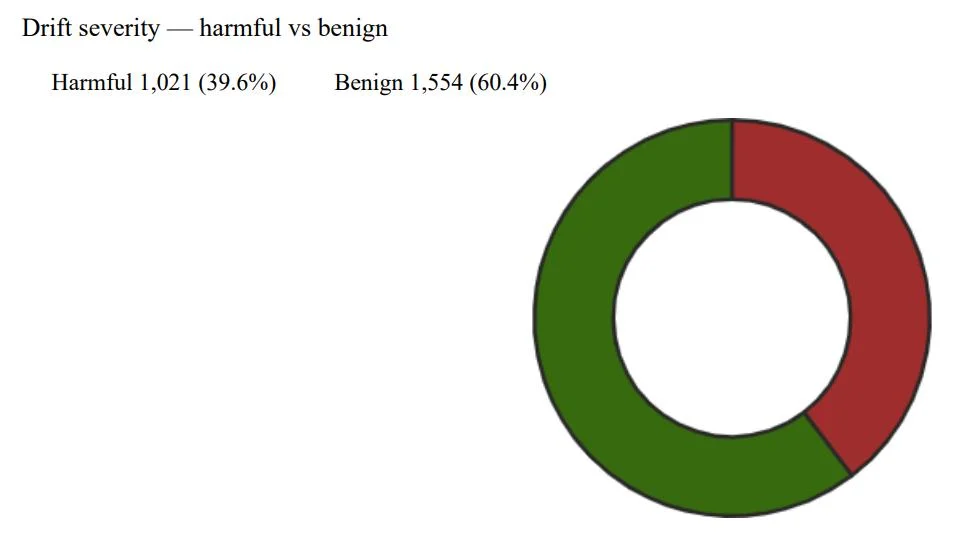
Fig. 4: Donut chart showing the split between harmful (39.6%) and benign (60.4%) drift events.
Fig. 4 shows the severity of drift effects as harmful and benign. The identified drift can be classified into harmful (1,021; 39.6%) and benign (1,554; 60.4%). Since presented drift cases have mostly been benign, there is no need to retrain the models for every detected drift, which is more convenient and cost-effective than alerting on every drift.
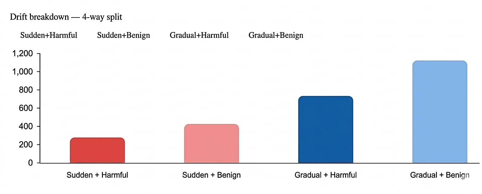
Fig. 5: Bar chart showing the four-way breakdown of drift events by type (sudden/gradual) and harmfulness (harmful/benign).
The bar chart in Fig. 5 analyzes all four combinations of drift type and harmfulness: sudden but harmful, sudden but not harmful, gradual but harmful, and gradual but not harmful. The biggest bar is gradual-but-not-harmful, indicating that most drifts in this dataset are gradual and easy to manage; the smallest is sudden-and-harmful.
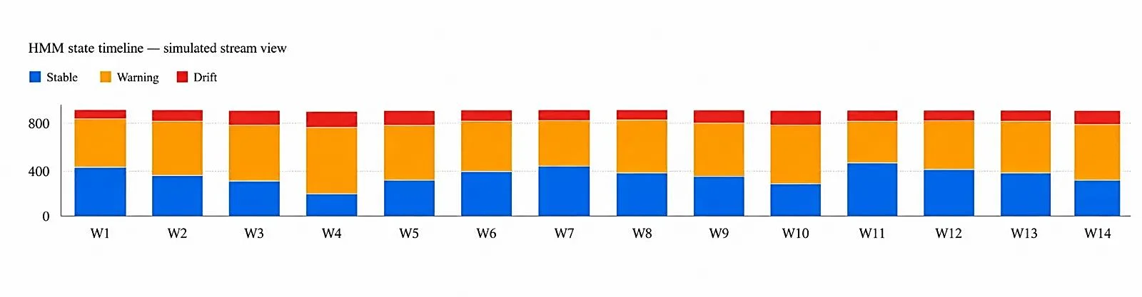
Fig. 6: HMM state timeline showing the distribution of stable, warning, and drift states across 14-time windows of the evaluation stream.
Fig. 6 illustrates the distribution of the three states — stable (blue), warning (orange), and drift (red) — within 14 windows (W1–W14). The initial windows (W1–W4) contain a greater proportion of stable state, whereas the latter windows have higher percentages of warning and drift due to gradual sensor deterioration; the increasing red-bar proportion in the latter windows is consistent with the physics of the dataset.
5. Discussion
5.1 Expected outcomes
Based on the experimental results and the design of the HDT system, a number of outcomes are expected to hold more broadly when the system is applied to other non-stationary data streams. The first expected outcome is that the three-state design genuinely improves the quality of drift detection compared to binary approaches, with the warning state appearing before most confirmed drift events. On the gas sensor dataset this was confirmed: the warning state occupied 44.2% of all time steps, and the state timeline showed warning consistently preceding drift-state stretches across all 14 windows, suggesting the HMM is picking up genuine early distributional signals rather than simply relabeling drift events after the fact.[19,20]
The second expected outcome is that the distinction between sudden and gradual drift carries real information about how urgent the response needs to be. Sudden drifts should tend to produce shorter warning phases and steeper KS rises, while gradual drifts should show longer build-ups. The results are consistent with this: the 714 sudden events are concentrated near the boundaries between sensor batches, where conditions changed quickly, while the 1,861 gradual events are spread across the longer within-batch degradation periods.
The third expected outcome is that the harmfulness score H(e) meaningfully separates events that require immediate model replacement from those that do not. The finding that 60.4% of confirmed drift events are benign suggests that if all 2,575 events had triggered full model retraining, roughly three out of every five retraining cycles would have been unnecessary.[21] Avoiding that overhead while still catching the 1,021 genuinely harmful events is the practical payoff of the harmfulness classification step.
The fourth expected outcome is that the HMM-based approach should generalize beyond the gas sensor dataset to other streams where drift develops gradually and early warning is valuable. The framework makes no domain-specific assumptions about the data — it only requires a sliding window from which the four features can be computed and a deployed model whose error rate can be monitored — making it applicable in principle to financial data, network traffic, medical monitoring, and other areas where concept drift is a known operational challenge.[22,23]
5.2 Technical limitations
Despite the encouraging results, the HDT system has technical limitations that should be acknowledged. The current implementation maps the 128-dimensional vectors from the gas sensor features to a scalar through the mean operation, performed over all sensors before applying the sliding-window analysis. This simplification ignores information related to individual sensor behaviour as well as correlations among sensors; any drift that impacts only a smaller number of sensors, or that manifests only through inter-sensor correlation rather than the mean, could go completely unnoticed. Future work should consider using HMMs directly on the multidimensional feature space, skipping dimensionality reduction.
A fixed window size w=100 is used across the whole experiment. The optimal window size is highly dependent on the speed of change of the incoming data's distribution: a too-narrow window is subject to noise, while a too-wide window is slow to catch on.[24] The current version of HDT does not adapt the window size based on experience; an adaptive windowing scheme, like ADWIN but for HMMs, should improve performance on different drift rates. The transition probabilities A and the emission-model parameters μi, Σi are estimated according to prior assumptions and then updated based on the observed stream through the Baum-Welch algorithm; the accuracy of this estimation relies on the length of the observed stream and the number of states within it, and a short or sparse stream can yield inaccurate parameters. Initialization of π and A also plays an important role.
It is assumed that the emission model follows a Gaussian distribution — a simple and mathematically convenient approach, but not always applicable.[25] For feature distributions with high skewness, multiple peaks, or large variances, this assumption will not hold, leading to incorrect state assignment; more sophisticated emission models such as a Gaussian mixture model or kernel density estimator could address this. The existing algorithm calculates only one statistic, KS, between a scalar current window and a scalar reference window; extending this to a true multivariate KS test is difficult because univariate KS statistics do not generalize cleanly to higher dimensions, so the model may fail to detect drift that exists only in the joint distribution of multiple features.
The existing HDT system also does not deal with recurring drift, where the data distribution returns to a previous distribution after cycling through several others. In such cases, the reference window Wref will already be drifted from the present data even though the current distribution resembles an earlier one. A smarter approach would involve maintaining a set of historical states and allowing the HMM to map the current data onto a historical state instead of always comparing to a fixed reference window.
6. Conclusions
This study presents an HDT-based drift detection system that not only detects the occurrence of drifts but also categorizes them by type. The system assumes that the stream evolves through three states (stable, warning, and drift) by applying an HMM, and the Viterbi algorithm calculates the maximum-likelihood sequence of states the stream passes through, determined from four statistical measures (mean, variance, KS statistic, and model error rate). Experiments on the UCI gas sensor array drift dataset identified 2,575 drift instances, of which 714 are sudden and 1,861 gradual; 1,021 instances were classified as harmful and the remaining 1,554 as benign. The experiment reveals that warning states appear before actual drifts, confirming that the model can be used as an early-warning detection system.
All ten methods discussed in the literature review share one common limitation that HDT effectively solves: they treat drift as a binary occurrence without temporal awareness, without classifying events, and without assessing severity. HDT incorporates all these features within a single framework while remaining highly computationally efficient.
Several promising directions can extend the HDT framework. First, the current scalar feature pipeline can be replaced by a fully multivariate HMM operating directly on the sensor feature matrix, enabling detection of drift that manifests only in inter-sensor correlations. Second, the fixed window size w can be replaced by an adaptive windowing mechanism that self-tunes based on the observed rate of state change. Third, the binary harmfulness criterion can be replaced by a continuous risk-scoring model that integrates downstream task performance loss. Fourth, the framework can be extended to handle recurring drift by maintaining a library of previously learned HMM emission models and matching the current stream to a historical regime. Fifth, the HDT system can be embedded into federated or edge-computing architectures for real-time drift monitoring in distributed sensor networks. Finally, the harmfulness and drift-type labels produced by HDT can serve as training signals for meta-learning approaches that learn to select the optimal adaptation strategy given the observed drift characteristics.
CRediT Author Contribution Statement
Bitan Misra: Conceptualization, Methodology, Supervision, Writing – Review & editing. Kailas Kunjumon: Data curation, Formal analysis, Investigation, Writing – original draft. Aksa Maria Paul: Investigation, Validation, Visualization, Writing – original draft. Mariya K Joby: Data curation, Resources, Validation, Writing – review & editing. Hemanth KS: Supervision, Project administration, Funding acquisition, Writing – review & editing. All authors have read and agreed to the published version of the manuscript.
Funding Declaration
This research did not receive any specific grant from funding agencies in the public, commercial, or not-for-profit sectors.
Data Availability Statement
Data used in this manuscript is available at https://www.kaggle.com/datasets/orvile/gas-sensor-array-drift-dataset.
Conflict of Interest
There is no conflict of interest.
Artificial Intelligence (AI) Use Disclosure
The authors declare that artificial intelligence (AI)-assisted tools were used only for language refinement, grammar improvement, and manuscript structuring purposes during the preparation of this work. All technical content, experimental implementation, results, and interpretations were independently developed and verified by the authors.
Supporting Information
Not applicable.
References
- [1] J. Lu, A. Liu, F. Dong, F. Gu, J. Gama, G. Zhang, Learning under concept drift: a review, IEEE Transactions on Knowledge and Data Engineering, 2019, 31, 2346-2363, doi: 10.1109/TKDE.2018.2876857.
- [2] J. Gama, I. Žliobaitė, A. Bifet, M. Pechenizkiy, A. Bouchachia, A survey on concept drift adaptation, ACM Computing Surveys, 2014, 46, 37, doi: 10.1145/2523813.
- [3] I. Žliobaitė, M. Pechenizkiy, J. Gama, An overview of concept drift applications, In: Japkowicz, N., Stefanowski, J. (eds) Big Data Analysis: New Algorithms for a New Society, Studies in Big Data, 2016, Springer, Cham, 16, doi: 10.1007/978-3-319-26989-4_4.
- [4] M. Baena-García, J. Campo-Ávila, R. Fidalgo, A. Bifet, R. Gavaldà, R. Morales-Bueno, Early drift detection method, in Fourth International Workshop on Knowledge Discovery from Data Streams, 2006, 6, 77-86.
- [5] D. N. Assis, V. M. A. Souza, ADWIN-U: adaptive windowing for unsupervised drift detection on data streams, Knowledge and Information Systems, 2025, 1-30, doi: 10.1007/s10115-025-02523-1.
- [6] Z. Zhang, H. Zhang, An online transfer learning model for intrusion detection using FT-Transformer and KSWIN-driven concept drift detection mechanism, 2024 5th International Conference on Computer Engineering and Application (ICCEA), 2024, 128-131, doi: 10.1109/ICCEA62105.2024.10603489.
- [7] D. Baehrens, T. Schroeter, S. Harmeling, M. Kawanabe, K. Hansen, K. R. Müller, How to explain individual classification decisions, The Journal of Machine Learning Research, 2010, 11, 1803-1831.
- [8] G. Montavon, S. Lapuschkin, A. Binder, W. Samek, K. R. Müller, Explaining nonlinear classification decisions with deep taylor decomposition, Pattern Recognition, 2017, 65, 211-222, doi: 10.1016/j.patcog.2016.11.008.
- [9] J. Z. Kolter, M. A. Maloof, Dynamic weighted majority: an ensemble method for drifting concepts, Journal of Machine Learning Research, 2007, 8, 2755-2790, doi: 10.1109/icdm.2003.1250911.
- [10] W. Wang, Q. Chen, X. He, L. Tang, Cooperative anomaly detection with transfer learning-based hidden Markov model in virtualized network slicing, IEEE Communications Letters, 2019, 23, 1534-1537, doi: 10.1109/LCOMM.2019.2923913.
- [11] S. Greco, B. Vacchetti, D. Apiletti, T. Cerquitelli, Unsupervised concept drift detection from deep learning representations in real-time, IEEE Transactions on Knowledge and Data Engineering, 2025, 37, 6232-6245, doi: 10.1109/TKDE.2025.3593123.
- [12] V. Losing, B. Hammer, H. Wersing, Incremental on-line learning: a review and comparison of state-of-the-art algorithms, Neurocomputing, 2018, 275, 1261-1274, doi: 10.1016/j.neucom.2017.06.084.
- [13] J. Komorniczak, P. Ksieniewicz, Unsupervised concept drift detection based on parallel activations of neural network, In International Workshop on Discovering Drift Phenomena in Evolving Landscapes, Springer Nature, 2024, 111-127, doi: 10.1007/978-3-031-82346-6_8.
- [14] L. M. Koch, C. F. Baumgartner, P. Berens, Distribution shift detection for the postmarket surveillance of medical AI algorithms: a retrospective simulation study, NPJ Digital Medicine, 2024, 7, 120, doi: 10.1038/s41746-024-01085-w.
- [15] L. Xiong, M. Wang, Z. Zhu, M. He, Y. Hou, X. Tang, Semi-supervised comparative learning compensation method for chemical gas sensor drift, Analytical and Bioanalytical Chemistry, 2024, 416, 6827-6838, doi: 10.1007/s00216-024-05577-2.
- [16] L. E. Baum, T. Petrie, G. Soules, N. Weiss, A maximization technique occurring in the statistical analysis of probabilistic functions of Markov chains, The Annals of Mathematical Statistics, 1970, 41, 164-171, doi: 10.1214/aoms/1177697196.
- [17] L. R. Rabiner, A tutorial on hidden Markov models and selected applications in speech recognition, Proceedings of the IEEE, 1989, 77, 257-286, doi: 10.1109/5.18626.
- [18] Gas Sensor Array Drift Dataset, 2012, https://archive.ics.uci.edu/dataset/224/gas+sensor+array+drift+dataset, accessed 18 May 2026.
- [19] T. M. T. Pham, K. Premkumar, M. Naili, J. Yang, Time to retrain? Detecting concept drifts in machine learning systems, 2025 IEEE/ACM 47th International Conference on Software Engineering: Software Engineering in Practice (ICSE-SEIP), 2025, 260-271, doi: 10.1109/ICSE-SEIP66354.2025.00029.
- [20] G. Hovakimyan, J. M. Bravo, Evolving strategies in machine learning: a systematic review of concept drift detection, Information, 2024, 15, 786, doi: 10.3390/info15120786.
- [21] S. S. Bagui, M. P. Khan, C. Valmyr, S. C. Bagui, D. Mink, Model retraining upon concept drift detection in network traffic big data, Future Internet, 2025, 17, 328, doi: 10.3390/fi17080328.
- [22] F. Liu, Z. Liu, X. Zhang, Z. Liu, Y. Liu, Machine learning-enhanced metal oxide gas sensor arrays: a review of selectivity and performance improvements, Sensor Review, 2025, 46, 629-647, doi: 10.1108/sr-08-2025-0639.
- [23] L. M. Ferrero, Continual contrastive learning for non-stationary data streams in autonomous systems, Journal of Multidisciplinary Knowledge, 2025, 5, 191-200, doi: 10.36676/jmk.v5.i2.97.
- [24] H. Mei, J. Peng, T. Wang, B. Zhang, F. Xuan, A semi-supervised domain adaptation for cross-gas concentration prediction with multi-target and bidirectional transfer for e-nose system, Sensors and Actuators B: Chemical, 2025, 450, 139242, doi: 10.1016/j.snb.2025.139242.
- [25] D. Lukats, O. Zielinski, A. Hahn, F. Stahl, A benchmark and survey of fully unsupervised concept drift detectors on real-world data streams, International Journal of Data Science and Analytics, 2025, 19, 1-31, doi: 10.1007/s41060-024-00620-y.
Publisher Note: The views, statements, and data in all publications solely belong to the authors and contributors. GR Scholastic is not responsible for any injury resulting from the ideas, methods, or products mentioned. GR Scholastic remains neutral regarding jurisdictional claims in published maps and institutional affiliations.
Open Access
This article is licensed under a Creative Commons Attribution-NonCommercial 4.0 International License, which permits the non-commercial use, sharing, adaptation, distribution and reproduction in any medium or format, as long as appropriate credit to the original author(s) and the source is given by providing a link to the Creative Commons License and changes need to be indicated if there are any. The images or other third-party material in this article are included in the article's Creative Commons License, unless indicated otherwise in a credit line to the material. If material is not included in the article's Creative Commons License and your intended use is not permitted by statutory regulation or exceeds the permitted use, you will need to obtain permission directly from the copyright holder. To view a copy of this License, visit: https://creativecommons.org/licenses/by-nc/4.0/
© The Author(s) 2026