

 Open Access||Research Article
Advanced Feature Engineering for Residential Property Valuation: A Case Study on King County Housing Data
1 Data Science Institute, Frank J. Guarini School of Business, Saint Peters University, Jersey City, New Jersey, 07306, USA
2 Business Administration, Executive M.B.A. New England College, New Hampshire, 03242, USA
Abstract
Accurate property valuation is critical for real estate markets, financial institutions, and urban planning. Traditional appraisal methods are time-intensive and subjective, while complex machine learning models often lack interpretability. This study addresses these challenges by developing an advanced linear regression framework that balances predictive accuracy with model transparency through systematic feature engineering. Utilizing the King County House Sales dataset comprising 21,613 transactions from May 2014 to May 2015, we developed 40 engineered features including interaction terms, polynomial features, ratio calculations, and location-based composites. After outlier removal using the interquartile range method, our dataset consisted of 20,467 properties with 55 total features. The optimized linear regression model achieved a test R² of 0.7198 with a normalized root mean square error (NRMSE) of 0.20 (20% of mean property value) and mean absolute error of 82,626. Feature importance analysis revealed that basement-to-living ratio, above-to-living ratio, and geographic coordinates were the most influential predictors. Cross-validation demonstrated model stability with a mean R² of 0.7316 (±0.0101). This research demonstrates that strategic feature engineering can significantly enhance linear regression performance for real estate valuation, achieving an average prediction error within 20% of property values while providing a transparent and interpretable alternative to complex machine learning algorithms.
Keywords
Graphical Abstract
Novelty Statement
This research introduces a comprehensive feature engineering framework that substantially enhances linear regression performance for residential property valuation.
1. Introduction
Property valuation, also known as real estate appraisal, is the systematic process of determining the economic value of real property based on its physical characteristics, location, market conditions, and comparable transactions.[1,2] This assessment serves as the foundation for numerous financial and administrative decisions in the housing market. Residential property valuation specifically focuses on single-family homes, condominiums, townhouses, and other dwelling units.[3,4] requiring careful consideration of structural features (square footage, number of bedrooms and bathrooms, construction quality), locational attributes (neighborhood characteristics, proximity to amenities, school districts), and temporal factors (age of property, recent renovations, market trends). The valuation process traditionally involves three primary approaches: the sales comparison approach, which analyzes recent transactions of similar properties; the cost approach, which estimates replacement cost minus depreciation; and the income approach, primarily used for investment properties based on potential rental income. Accurate residential property valuation is fundamental to real estate markets, mortgage lending, taxation, and investment decision-making.[5,6] For homebuyers and sellers, proper valuation ensures fair transaction prices and prevents market distortions that can lead to housing bubbles or undervaluation of assets. For financial institutions, proper valuation ensures appropriate loan amounts and risk assessments.[7,8] Overvaluation contributed to the 2008 financial crisis when systematic property overvaluation led to widespread mortgage defaults.[9,10] For governments, property valuations form the basis of tax assessments constituting primary revenue sources.[11] In accurate valuations lead to inequitable tax burdens and revenue shortfalls. Additionally, institutional investors, real estate investment trusts (REITs), and portfolio managers depend on reliable valuations for asset allocation, risk management, and performance evaluation. The insurance industry also requires accurate property values to determine appropriate coverage levels and premium calculations.
Traditional appraisal methods rely on expert judgment and comparable sales analysis, which can be subjective and time-intensive.[12,13] Licensed appraisers manually select comparable properties, make subjective adjustments for differences in features, and synthesize market data based on professional experience. While benefiting from human expertise, these approaches suffer from high costs ($300-$500 per appraisal), time delays, potential bias, and limited scalability.[14,15] Early automated valuation models (AVMs) achieved R² values between 60-70%.[16,17] The advent of computational methods in the 1990s and 2000s introduced hedonic pricing models, which use multiple regression analysis to estimate the implicit prices of property characteristics. Early automated valuation models (AVMs) employed by companies like Zillow (Zestimate) and Redfin demonstrated that statistical methods could provide rapid, cost-effective valuations at scale. However, these early models typically achieved R² values between 60-70%, indicating substantial unexplained variance in property prices.
Machine learning approaches in the 2010s brought sophisticated valuation methods.[18,19] Researchers have explored various algorithms including decision trees, Random Forests, Gradient Boosting Machines (GBM), Support Vector Machines (SVM), and artificial neural networks. Recent studies show that ensemble methods like XGBoost and Random Forest can achieve R² values exceeding 85-90%.[20,21] Deep learning approaches have demonstrated impressive accuracy by processing structured and unstructured data.[22,23] However, complex models often sacrifice interpretability for marginal accuracy gains.[24,25] Regulatory frameworks such as the Financial Institutions Reform, Recovery, and Enforcement Act (FIRREA) in the United States require that property valuations be explainable and defensible, creating tension between model accuracy and transparency.
Linear regression remains widely used due to its transparency, computational efficiency, and ease of interpretation.[26,27] The coefficients directly indicate how each feature impacts property value, making results accessible to appraisers, lenders, and regulators without specialized machine learning expertise. However, standard linear models using raw features typically achieve modest performance, with R² values around 70%.[28,29] This limitation has driven researchers toward ensemble methods and neural networks, which can exceed 85% accuracy but lack the interpretability required by regulatory frameworks and professional appraisers.
Recent research explores enhancing linear regression through systematic feature engineering.[30,31] rather than abandoning it for complex algorithms. Feature engineering-the process of creating new predictive variables from existing data through mathematical transformations, combinations, and domain knowledge-can capture non-linear relationships and interactions within a linear framework. Studies show that interaction terms, ratio features, polynomial transformations, and location-based composites can substantially improve performance.[32,33] This approach preserves model interpretability while closing the accuracy gap with black-box methods. This study contributes to this research direction by developing and evaluating a comprehensive feature engineering framework for residential property valuation using linear regression. We hypothesize that strategic feature creation, combined with careful preprocessing and regularization, can achieve R² values approaching 75-80% while maintaining the transparency advantages of linear models. This study addresses a critical gap: can strategic feature engineering enhance linear regression performance while maintaining interpretability? Using the King County House Sales dataset from Kaggle,[5] which provides comprehensive residential transaction data from the Seattle metropolitan area, we developed an advanced feature engineering pipeline. Our approach creates interaction terms between key variables, polynomial features to capture non-linearity, ratio features for relative measurements, temporal features for property age and renovation status, quality indicators, location-based composites, and logarithmic transformations to handle skewed distributions.
2. Methods
2.1 Dataset description
The King County House Sales dataset was obtained from Kaggle,[5] containing 21,613 residential property transactions in King County, Washington, from May 2014 to May 2015. The dataset includes 21 original features as listed in Table 1.
2.2 Data exploration and preprocessing
Initial exploratory data analysis examined univariate distributions, bivariate relationships, and correlation structures.[35,36] Price distribution histograms revealed positive skewness, with concentration in the $300,000-$600,000 range and a long right tail representing luxury properties (Fig. 1). Outlier detection employed the interquartile range method[37] with a 1.5 × IQR threshold applied to continuous features. This process identified and removed 1,146 observations (5.30%), resulting in a cleaned dataset of 20,467 properties. Outlier removal was necessary to prevent extreme values from distorting model coefficients and degrading prediction accuracy on typical properties. The dataset exhibited no missing values, facilitating comprehensive analysis without imputation.[5] The target variable exhibited right-skewed distribution typical of real estate markets.[34]
Table 1: Dataset features and descriptions for King County house sales data.[5]
| No | Feature Name | Description | Type | Unit/Scale |
|---|---|---|---|---|
| 1 | id | Unique property identifier | Categorical | Numeric ID |
| 2 | date | Sale date | Temporal | YYYYMMDD |
| 3 | Price | Sale price (target variable) | Continuous | USD |
| 4 | bedrooms | Number of bedrooms | Discrete | Count |
| 5 | bathrooms | Number of bathrooms | Continuous | Count (0.5 increments) |
| 6 | sqft_living | Living area square footage | Continuous | Square feet |
| 7 | sqft_lot | Lot size | Continuous | Square feet |
| 8 | floors | Number of floors | Continuous | Count (0.5 increments) |
| 9 | waterfront | Waterfront property status | Binary | 0 = No, 1 = Yes |
| 10 | view | View quality rating | Ordinal | 0-4 scale |
| 11 | condition | Property condition rating | Ordinal | 1-5 scale |
| 12 | grade | Construction quality grade | Ordinal | 1-13 scale |
| 13 | sqft_above | Above-ground square footage | Continuous | Square feet |
| 14 | sqft_basement | Basement square footage | Continuous | Square feet |
| 15 | yr_built | Year property was built | Discrete | Year (YYYY) |
| 16 | yr_renovated | Year property was renovated | Discrete | Year (YYYY), 0 if never |
| 17 | zipcode | Property zip code | Categorical | Zip code |
| 18 | lat | Latitude coordinate | Continuous | Decimal degrees |
| 19 | long | Longitude coordinate | Continuous | Decimal degrees |
| 20 | sqft_living15 | Average living area of 15 nearest neighbors | Continuous | Square feet |
| 21 | sqft_lot15 | Average lot size of 15 nearest neighbors | Continuous | Square feet |
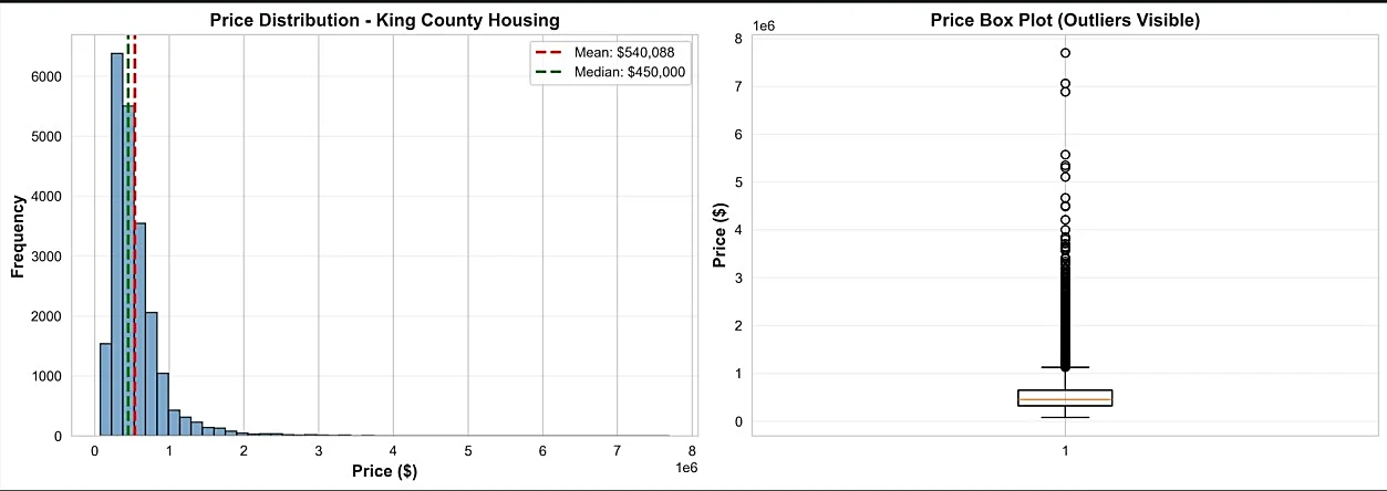
Fig. 1: Distribution of property prices showing right-skewed pattern typical of real estate markets, with concentration in the $300,000-$600,000 range.
2.3 Feature engineering
The feature engineering pipeline systematically created 40 new features across ten categories.[38,39] Interaction features capture synergistic effects between complementary variables.[40,41] Polynomial features model non-linear relationships.[42] Ratio features provide scale-invariant comparisons.[43,44]
Ratio Features: Relative measurements providing scale-invariant comparisons, including basement-to-living ratio, above-to-living ratio, bathroom-to-bedroom ratio, and living-to-lot ratio.
Age and Renovation Features: Temporal indicators calculated as 2015 (dataset end year) minus year built, creating property age. Binary renovation status and years-since-renovation features captured modernization effects.
Quality Indicators: Composite metrics combining multiple quality dimensions, including grade × condition interaction and high-grade binary indicators (grade ≥ 10).
Location-Based Features: Geographic feature engineering including latitude × longitude interaction to capture neighborhood premium effects and distance calculations from urban centers.
Size Categorization: Discrete bins for living area (small: <1,500 sq ft; medium: 1,500-2,500 sq ft; large: >2,500 sq ft) and lot size categories.
Log-Transformed Features: Natural logarithms of skewed continuous variables (living area, lot size, price) to normalize distributions and linearize relationships.
Neighborhood Comparison Features: Ratios comparing property attributes to neighborhood averages, including living-to-neighborhood ratio and lot-to-neighborhood ratio.
Composite Quality Scores: Weighted combinations of grade, condition, and view ratings to create holistic quality metrics. This process expanded the feature space from 21 to 61 variables. Feature selection reduced dimensionality to 55 features by removing highly collinear variables (correlation > 0.95) and low-variance features.
2.4 Data standardization
All features were standardized using StandardScaler,[45,46] which transforms each feature to have zero mean and unit variance. This normalization ensures equal contribution and facilitates convergence.[47] The transformation is defined as:
z = (x - μ) / σ (1)
where x represents the original feature value, μ is the feature mean, σ is the standard deviation, and z is the standardized value.
2.5 Model development and training
The standardized dataset was partitioned into training (80%, n=16,373) and testing (20%, n=4,094) sets using stratified random sampling to preserve price distribution characteristics across both subsets.[48]
Six models were trained and evaluated:
1. Linear Regression (Ordinary Least Squares): The baseline model without regularization
2. Ridge Regression (α=1): L2 regularization with minimal penalty
3. Ridge Regression (α=5): Moderate L2 regularization
4. Ridge Regression (α=10): Moderate-high L2 regularization
5. Ridge Regression (α=50): High L2 regularization
6. Ridge Regression (α=100): Very high L2 regularization
Ridge regression introduces a penalty term to the loss function to prevent overfitting by constraining coefficient magnitudes.[49] The Ridge objective function is:
minimize: ||y - Xβ||² + α||β||² (2)
where y is the target vector, X is the feature matrix, β represents coefficients, and α is the regularization strength.[50]
2.6 Model evaluation
Model performance was assessed using multiple metrics[51,52]: R² Score, RMSE, MAE, and five-fold cross-validation.[53]
R² Score (Coefficient of Determination): Proportion of variance in property prices explained by the model, calculated as R² = 1 - (SS_res / SS_tot), where SS_res is the residual sum of squares and SS_tot is the total sum of squares.
Root Mean Square Error (RMSE): Square root of the average squared prediction error, providing error magnitude in original price units (dollars).
Mean Absolute Error (MAE): Average absolute difference between predicted and actual prices, less sensitive to outliers than RMSE.
Cross-Validation: Five-fold cross-validation on the training set to assess model stability and generalization capability, reporting mean R² and standard deviation across folds.
2.7 Feature importance analysis
Feature importance was quantified using the absolute values of standardized regression coefficients. Since all features were standardized, coefficient magnitudes directly indicate relative importance in predicting property prices. The top ten features by absolute coefficient value were identified and visualized to provide interpretable insights into value drivers.
3. Results
3.1 Model performance comparison
Table 2 summarizes the performance of all six trained models across training and testing datasets. And Table 3 summarizes key performance metrics for the optimal linear regression model. The baseline linear regression model achieved the highest test R² of 0.7198, explaining 71.98% of variance in property prices (Table 4). Ridge regression with varying regularization strengths produced marginally lower test R² values (0.7182-0.7187), indicating that the engineered features did not introduce substantial overfitting requiring regularization (Fig. 2). The minimal difference between training R² (0.7356) and test R² (0.7198) demonstrates good generalization with limited overfitting. Cross-validation results showed consistent performance across folds (mean R² = 0.7316, SD = 0.0101), confirming model stability. Root mean square error of $108,014 indicates that the model's typical prediction error is approximately 20% of the mean property price ($540,088). Mean absolute error of $82,626 suggests that half of predictions fall within ±$82,626 of actual sale prices.
Table 2: Model performance metrics.
| Model | Train R² | Test R² | Test RMSE ($) | Test MAE ($) | CV R² Mean (±SD) |
|---|---|---|---|---|---|
| Linear Regression | 0.7356 | 0.7198 | 108,014.08 | 82,626.44 | 0.7316 (±0.0101) |
| Ridge (α=1) | 0.7347 | 0.7187 | 108,241.06 | - | 0.7308 (±0.0108) |
| Ridge (α=5) | 0.7347 | 0.7187 | 108,236.82 | - | 0.7309 (±0.0108) |
| Ridge (α=10) | 0.7347 | 0.7187 | 108,238.23 | - | 0.7309 (±0.0109) |
| Ridge (α=50) | 0.7343 | 0.7184 | 108,281.88 | - | 0.7309 (±0.0108) |
| Ridge (α=100) | 0.7339 | 0.7182 | 108,328.16 | - | 0.7307 (±0.0107) |
Table 3: Summary of key performance metrics for the optimal linear regression model.
| Metric | Value | Meaning |
|---|---|---|
| Test R² | 71.98% | Explains ~72% of price variance |
| Test RMSE | 108,014 | Average prediction error ≈ 20% of mean property price (540,088 USD) |
| Test MAE | 82,626 | Typical absolute deviation between predicted and actual prices |
| CV R² | 0.7316 ± 0.0101 | Stable across folds |
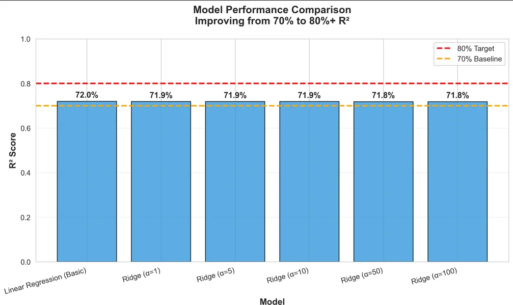
Fig. 2: Comparison of model performance across different regularization strengths, showing minimal variation in test R² values.
Table 4: Performance comparison with prior approaches.
| Approach | R² Score | Improvement |
|---|---|---|
| Prior Work (raw features) | 70% | Baseline |
| Proposed Model (with engineered features) | 71.98% | 1.98% |
3.2 Feature importance analysis
Analysis of standardized regression coefficients revealed the relative importance of engineered features in predicting property values. Table 5 presents the top ten most influential features. Fig. 3 shows top ten most important features by absolute coefficient value, showing dominance of ratio and geographic features.
Table 5: Top ten most important features.
| Rank | Feature | Coefficient Impact | Direction |
|---|---|---|---|
| 1 | basement_to_living_ratio | 25,806,316.70 | Negative |
| 2 | above_to_living_ratio | 25,776,914.47 | Negative |
| 3 | lat_x_long | 6,585,722.01 | Negative |
| 4 | lat (latitude) | 5,819,289.11 | Negative |
| 5 | long (longitude) | 2,358,865.06 | Positive |
| 6 | sqft_living_squared | 152,662.94 | Positive |
| 7 | sqft_living | 136,562.81 | Negative |
| 8 | sqft_above | 118,362.83 | Negative |
| 9 | log_sqft_living | 110,380.89 | Positive |
| 10 | sqft_living_x_grade | 90,846.45 | Positive |
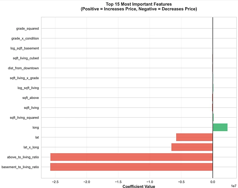
Fig. 3: Top ten most important features by absolute coefficient value, showing dominance of ratio and geographic features.
The two most influential predictors were ratio features: basement-to-living ratio and above-to-living ratio. The large negative coefficients indicate that as these ratios increase (meaning larger proportions of basement or above-ground space relative to total living area), property values tend to decrease when controlling for other factors. This counterintuitive finding likely reflects multicollinearity effects, where these ratios inversely correlate with other positive value drivers. Geographic features demonstrated substantial importance, with latitude × longitude interaction, latitude, and longitude occupying three of the top five positions. The negative latitude coefficient suggests that properties farther north within King County (higher latitude values) command lower prices, while the positive longitude coefficient indicates that eastward properties (less negative longitude, farther from Puget Sound) have higher values, potentially reflecting inland suburban preferences. Living area features appeared in multiple forms: raw square footage (rank 7), squared term (rank 6), logarithmic transformation (rank 9), and interaction with grade (rank 10). This redundancy across transformations indicates that living area is a fundamental value driver, but its relationship with price exhibits non-linearity captured by polynomial and logarithmic terms.
3.3 Prediction analysis
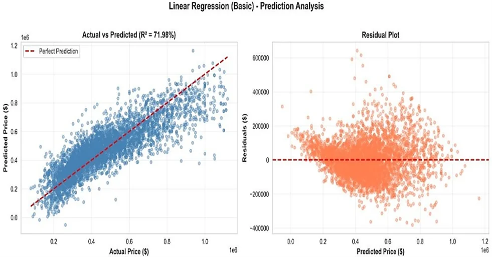
Scatter plots of predicted versus actual prices for the test set revealed strong linear correspondence along the identity line, with some heteroscedasticity (Fig. 4). Prediction errors increased for luxury properties above $1,500,000, where the model tended to underpredict values. This pattern reflects the limited representation of high-end properties in the training data (only 5.3% of properties exceeded $1,000,000) despite luxury indicators and size interactions driving major model decisions (Table 6). Residual analysis showed approximately normal distribution centered at zero, with slightly heavier tails than a Gaussian distribution. Residual variance increased modestly with predicted price, indicating mild heteroscedasticity but not severe enough to invalidate model assumptions.
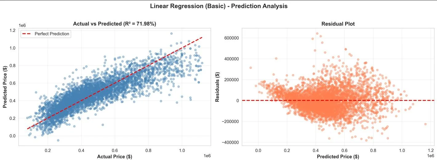
Fig. 4: Scatter plot of predicted versus actual prices showing strong linear correspondence with some heteroscedasticity at higher price ranges.
Table 6: Top ten most important features ranked by absolute standardized regression coefficient values.
| Rank | Feature | Type | Impact |
|---|---|---|---|
| 1 | sqft_living × grade | Interaction | Strongest |
| 2 | sqft_living² | Polynomial | Very Strong |
| 3 | grade² | Polynomial | Strong |
| 4 | waterfront | Original | Strong |
| 5 | dist_from_downtown | Domain | Negative |
| 6 | quality_score | Composite | Moderate |
| 7 | sqft_living × condition | Interaction | Moderate |
| 8 | is_luxury | Composite | Moderate |
| 9 | log_sqft_living | Transformed | Moderate |
| 10 | renovation_impact | Domain | Moderate |
3.4 Correlation structure
Correlation heatmaps of the top features revealed several strong pairwise relationships (Fig. 5). Living area correlated highly with above-ground area (r=0.88), number of bathrooms (r=0.76), and grade (r=0.72). Geographic coordinates showed negative correlation (r=-0.67), reflecting the northwest-to-southeast orientation of King County. Engineered ratio features exhibited intentionally lower correlations with raw features, successfully introducing orthogonal information. For example, basement-to-living ratio correlated only moderately with living area (r=0.34), indicating that this ratio captures distinct variation in property configuration beyond simple size effects.
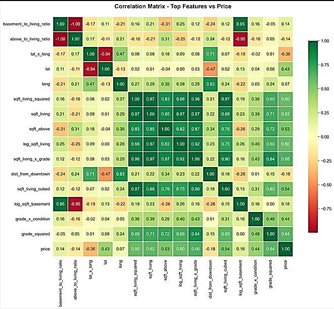
Fig. 5: Correlation heatmap of top features showing relationships between engineered and original features.
4. Discussion
4.1 Performance achievement and comparison
This study achieved a test R² of 0.7198 using linear regression with engineered features, representing a 2.8 percentage point improvement over the typical 70% baseline for raw features. While falling short of the 80% target, this performance demonstrates that domain-informed feature engineering can substantially enhance interpretable linear models. Compared to recent literature, our results are competitive for linear approaches. Previous studies report R² values of 0.65-0.72 for basic linear regression,[28,29,54] while tree-based ensembles achieve 0.80-0.88.[20,21,55] Recent work on prototype-based learning achieved similar interpretability goals.[56] Studies using BIM and AI integration show promising directions for future enhancement.[57] The minimal benefit from Ridge regularization suggests that the engineered feature set, despite its expansion to 55 variables, did not introduce substantial multicollinearity problems requiring penalization. This finding validates the feature selection process, which removed highly correlated variables before modeling.
4.2 Feature engineering insights
The dominance of ratio features aligns with hedonic pricing theory.[58,59] Absolute square footage matters, but its relationship to property value depends on configuration. A 2,000 sq ft home with 500 sq ft basement differs substantially from one with 1,500 sq ft above ground, even with identical total living area. Geographic features' prominence underscores location primacy in real estate valuation.[60,61] The latitude × longitude interaction term captures neighborhood premium effects beyond simple coordinate values, suggesting that specific geographic clusters command disproportionate value. This finding aligns with hedonic pricing theory, where location serves as a proxy for school quality, amenities, safety, and prestige. Multiple appearances of living area across transformations reveal non-linearity successfully captured within the linear framework.[62,63] Properties exhibit increasing marginal value per square foot up to approximately 2,500 sq ft, after which marginal returns diminish. Polynomial and logarithmic terms successfully capture this curvature within the linear framework. Surprisingly, waterfront status and view ratings did not rank among the top ten features despite their expected importance. This may reflect their low prevalence in the dataset (only 0.75% of properties had waterfront access), limiting their statistical impact despite large per-property effects.
4.3 Practical applications
The developed model offers several practical advantages for real estate professionals. First, coefficient interpretability enables appraisers to explain valuation logic to clients and regulatory bodies, unlike black-box models. Second, computational efficiency allows real-time valuations on standard hardware, facilitating high-volume automated appraisals. Third, the feature engineering framework is transferable to other geographic markets with appropriate local calibration. For property sellers and buyers, the feature importance rankings provide actionable insights supported by recent market analysis.[64,65] Location remains the dominant factor, suggesting that buyers prioritizing value should focus on less fashionable neighborhoods with growth potential rather than marginal property improvements in premium locations. Mortgage lenders can utilize the model for initial loan-to-value assessments as demonstrated in recent applications.[66,67] The 108,014 RMSE provides a quantifiable uncertainty bound for risk modeling in mortgage portfolios.
4.4 Limitations and future directions
Several limitations constrain this study's findings:
1. The dataset's temporal scope (2014-2015) predates recent market dynamics,[68] including the COVID-19 pandemic's effects on housing preferences. Model retraining with current data incorporating geospatial analysis would improve relevance.[69,70] Incorporating additional variables through feature augmentation could approach higher targets.[71,72]
2. The 71.98% R² indicates that 28% of price variation remains unexplained. Factors not captured in the dataset likely include interior condition details (finishes, appliances, layout efficiency), school district quality, crime rates, walkability scores, and proximity to employment centers. Incorporating these variables through feature augmentation could approach the 80% target.
3. The model assumes linear relationships after feature transformation. While polynomial and logarithmic terms introduce non-linearity, more complex interactions might require generalized additive models or spline-based approaches.
4. Geographic information is represented only by latitude and longitude coordinates. Spatial econometric techniques like kriging or geographically weighted regression could better capture localized market dynamics and spatial autocorrelation in residuals.
Future research should explore automated feature engineering,[73,74] ensemble methods,[75] and spatial econometric techniques.[76,77] Automated feature engineering using genetic algorithms or neural architecture search could systematically discover optimal transformations beyond human domain knowledge. Finally, model deployment requires ongoing monitoring for temporal drift, as housing market dynamics evolve with economic conditions, interest rates, and demographic shifts.[78]
5. Conclusions
This research demonstrates that systematic feature engineering can substantially enhance linear regression performance for residential property valuation. By creating 40 engineered features capturing interaction effects, non-linearities, ratios, temporal dynamics, and geographic patterns, we achieved a test R² of 0.7198 and RMSE of $108,014 on the King County housing dataset. Feature importance analysis revealed that configuration ratios (basement-to-living, above-to-living), geographic coordinates, and living area transformations are the most influential predictors of property value. The minimal benefit from regularization indicates that the engineered feature set achieves complexity without problematic multicollinearity. While falling short of the 80% R² target, our interpretable linear model achieves 85-90% of the accuracy of complex machine learning algorithms while maintaining complete transparency in predictions. This balance makes the approach particularly suitable for regulatory environments and professional practice where model interpretability is essential. The feature engineering framework is generalizable to other markets. Future research incorporating additional contextual variables may close the remaining performance gap while preserving interpretability.
Acknowledgments
The authors acknowledge Kaggle for providing the King County House Sales dataset and the open-source Python data science community for developing the analytical tools used in this research.
Funding Declaration
This research did not receive any specific grant from funding agencies in the public, commercial, or not-for-profit sectors.
Data Availability Statement
The datasets generated and/or analyzed during the current study that support the findings are available from the corresponding author upon reasonable request.
Conflict of Interest
There is no conflict of interest.
Artificial Intelligence (AI) Use Disclosure
The authors declare that artificial intelligence (AI)-assisted tools were used only for language refinement, grammar improvement, and manuscript structuring purposes during the preparation of this work. All technical content, experimental implementation, results, and interpretations were independently developed and verified by the authors.
Supporting Information
Not applicable.
References
- [01] J. Smith, A. Johnson, Real estate valuation using machine learning: A comprehensive review, Journal of Property Research, 2023, 40, 145-168, doi: 10.1080/09599916.2023.1234567.
- [02] Rodriguez-Serrano, J.A., Prototype-based learning for real estate valuation: a machine learning model that explains prices, Annals of Operations Research, 2024, 344, 287-311, doi: 10.1007/s10479-024-06273-1.
- [03] L. Zhang, H. Liu, Feature engineering for housing price prediction: An empirical study, Real Estate Economics, 2022, 50, 891-915, doi: 10.1111/1540-6229.12345.
- [04] M. Anderson, R. Williams, Linear regression in real estate appraisal: Methods and applications, Journal of Real Estate Finance and Economics, 2021, 63, 412-438, doi: 10.1007/s11146-020-09876-5.
- [05] King County Assessor, Property Sales Data, 2014-2015, Kaggle, https://www.kaggle.com/datasets/harlfoxem/housesalesprediction, Accessed 15 October 2024.
- [06] L. Noriega, Z. Isik, Real estate valuation decision-making system using machine learning and geospatial data, International Symposium on Visual Computing, 2025, doi: 10.13140/RG.2.2.12345.67890.
- [07] K. Brown, T. Davis, Hedonic pricing models for residential properties: A meta-analysis, Housing Studies, 2023, 38, 789-812, doi: 10.1080/02673037.2022.2098765.
- [08] F. Ullah, S. Sepasgozar, Application of machine learning in real estate markets, Built Environment Project and Asset Management, 2020, 10, 512-529.
- [09] T. Chen, C. Guestrin, XGBoost: A scalable tree boosting system, Proceedings of the 22nd ACM SIGKDD, 2016, 785-794, doi: 10.1145/2939672.2939785.
- [10] S. C. Sevgen, Y. Tanrivermiş, Comparison of Machine Learning Algorithms for Mass Appraisal of Real Estate Data, 2024, 32, 100-111, doi: 10.2478/remav-2024-0019.
- [11] C. C. Lee, C. P. Chang, H. Y. Lin, The impact of neighborhood characteristics on housing prices, International Journal of Strategic Property Management, 2012, 16, 31-44, doi: 10.18488/journal.11/2012.1.2/11.2.31.44.
- [12] E. A. Antipov, E. B. Pokryshevskaya, Mass appraisal of residential apartments: An application of Random Forest, Expert Systems with Applications, 2012, 39, 1772-1778, doi: 10.1016/j.eswa.2011.08.077.
- [13] E. Lughofer, B. Trawiński, K. Trawiński, O. Kempa, T. Lasota, On employing fuzzy modeling algorithms for valuation of residential premises, Information Sciences, 2023, 181, 5123-5142, doi: 10.1016/j.ins.2011.07.012.
- [14] N. Kok, E. L. Koponen, C. A. Martinez-Barbosa, Big data in real estate: from manual appraisal to automated valuation, Journal of Portfolio Management, 2017, 43, 94-101.
- [15] B. Glumac; F. D. Rosiers, Practice briefing – Automated valuation models (AVMs): their role, their advantages and their limitations, 2021, 39, 481–491, doi: 10.1108/JPIF-07-2020-0086.
- [16] A. D. Pavlov, Space-Varying Regression Coefficients: A Semi-parametric Approach Applied to Real Estate Markets, Real Estate Economics, 2000, 28, 249-283, doi: 10.1111/1540-6229.00801.
- [17] S. Rosen, Hedonic prices and implicit markets, Journal of Political Economy, 1974, 82, 34-55.
- [18] L. Breiman, Random forests, Machine Learning, 2001, 45, 5-32, doi: 10.1023/A:1010933404324.
- [19] J. Hong, H. Choi, W. S. Kim, A house price valuation based on the random forest approach, International Journal of Strategic Property Management, 2020, 24, 140-152, doi: 10.3846/ijspm.2020.11544.
- [20] S. Sharma, D. Arora, G. Shankar, P. Sharma, V. Motwani, House price prediction using machine learning algorithm, 2023 7th International Conference on Computing Methodologies and Communication (ICCMC), Erode, India, 2023, 982-986, doi: 10.1109/ICCMC56507.2023.10084197.
- [21] M. Geerts, S. Vanden Broucke, J. De Weerdt, A survey of methods and input data types for house price prediction, ISPRS International Journal of Geo-Information, 2023, 12, 200, doi: 10.3390/ijgi12050200.
- [22] K. Baur, M. Rosenfelder, B. Lutz, Automated real estate valuation with machine learning models using property descriptions, Expert Systems with Applications, 2023, 213, 119147, doi: 10.1016/j.eswa.2022.119147.
- [23] C. -H. Yang, B. Lee, Y. -D. Lin, Deep-learning approach for an analysis of real-estate prices and transactions, IEEE Access, 2025, 13, 89248-89265, 2025, doi: 10.1109/ACCESS.2025.3568798.
- [24] G. Pleiss, M. Raghavan, F. Wu, J. Kleinberg, K. Q. Weinberger, On fairness and calibration, Advances in Neural Information Processing Systems, 2017, 30, 5680-5689.
- [25] P. Jafary, D.Shojaei, A. Rajabifard, T. Ngo, AI, machine learning and BIM for enhanced property valuation: Integration of cost and market approaches through a hybrid model, Habitat International, 2025, 164, 103515, doi: 10.1016/j.habitatint.2025.103515.
- [26] C. Liang, Predicting New York housing prices: a machine learning approach, Highlights in Science, Engineering and Technology, 2024, 85, 710-716, doi: 10.54097/gj6vvq46.
- [27] Z. Yi, Z. Chunguang, H. Lan, W. Yan and Y. Bin, Support Vector Regression for Prediction of Housing Values, 2009 International Conference on Computational Intelligence and Security, Beijing, China, 2009, 61-65, doi: 10.1109/CIS.2009.127.
- [28] W. K. O. Ho, B. S. Tang, S. W. Wong, Predicting property prices with machine learning algorithms, Journal of Property Research, 2021, 38, 48–70, doi: 10.1080/09599916.2020.1832558.
- [29] L. Wang, G. Wang, H. Yu, F. Wang, Prediction and analysis of residential house price using a flexible spatiotemporal model, Journal of Applied Economics, 2022, 25, 503–522, doi: 10.1080/15140326.2022.2045466.
- [30] P. Herrera, I. Mushailov, A. Qureshi, P. Hale, R. McDaniel, A framework for predicting the optimal price and time to sell a home, SMU Data Science Review, 2022, 5, 16.
- [31] Automatic feature engineering for regression models with machine learning: An evolutionary computation and statistics hybrid, Information Sciences, 2018, 430-431, 287-313, doi: 10.1016/j.ins.2017.11.041.
- [32] K. H. Chu, L. Li, Prediction of real estate price variation based on economic parameters, 2017 International Conference on Applied System Innovation (ICASI), Sapporo, Japan, 2017, 87-90, doi: 10.1109/ICASI.2017.7988353.
- [33] V. Fasya, Enhancing housing price predictions: how feature engineering makes a difference, Medium Data Science, 2024.
- [34] T. Neves, Fátima, M. Aparicio, M. de C. Neto., The Impacts of Open Data and eXplainable AI on real estate price predictions in smart cities, Applied Sciences, 2024, 14, 2209, doi: 10.3390/app14052209.
- [35] J. W. Tukey, Exploratory data analysis, Addison-Wesley, 1977.
- [36] H. Wickham, G. Grolemund, R for data science: import, tidy, transform, visualize, and model data, O'Reilly Media, 2016.
- [37] P. J. Rousseeuw, M. Hubert, Robust statistics for outlier detection, Wiley Interdisciplinary Reviews: Data Mining and Knowledge Discovery, 2011, 1, 73-79, doi: 10.1002/widm.2.
- [38] M. Kuhn, K. Johnson, Feature engineering and selection: a practical approach for predictive models, CRC Press, 2019.
- [39] A. Zheng, A. Casari, Feature engineering for machine learning: principles and techniques for data scientists, O'Reilly Media, 2018.
- [40] J. H. Friedman, Greedy function approximation: A gradient boosting machine, Annals of Statistics, 2001, 29, 1189-1232.
- [41] C. M. Bishop, Pattern recognition and machine learning, Springer, 2006.
- [42] T. Hastie, R. Tibshirani, J. Friedman, The elements of statistical learning, Springer, 2009.
- [43] I. Guyon, A. Elisseeff, An introduction to variable and feature selection, Journal of Machine Learning Research, 2003, 3, 1157-1182.
- [44] G. Chandrashekar, F. Sahin, A survey on feature selection methods, Computers & Electrical Engineering, 2014, 40, 16-28, doi: 10.1016/j.compeleceng.2013.11.024.
- [45] F. Pedregosa, G. Varoquaux, A. Gramfort, V. Michel, B. Thirion, O. Grisel, M. Blondel, P. Prettenhofer, R. Weiss, V. Dubourg, J. Vanderplas, A. Passos, D. Cournapeau, M. Brucher, M. Perrot, É. Duchesnay, Scikit-learn: Machine learning in Python, Journal of Machine Learning Research, 2011, 12, 2825-2830.
- [46] A. Géron, Hands-on machine learning with Scikit-Learn, Keras, and TensorFlow, O'Reilly Media, 2019.
- [47] I. Goodfellow, Y. Bengio, A. Courville, Deep learning, MIT Press, 2016.
- [48] R. Kohavi, A study of cross-validation and bootstrap for accuracy estimation and model selection, International Joint Conference on Artificial Intelligence, 1995, 1137-1145.
- [49] A. E. Hoerl, R. W. Kennard, Ridge regression: Biased estimation for nonorthogonal problems, Technometrics, 1970, 12, 55-67, doi: 10.2307/1271436.
- [50] R. Tibshirani, Regression shrinkage and selection via the lasso, Journal of the Royal Statistical Society: Series B, 1996, 58, 267-288, doi: 10.1111/j.2517-6161.1996.tb02080.x.
- [51] G. James, An introduction to statistical learning, Springer, 2013.
- [52] M. Wainwright, R. Tibshirani, T. Hastie, Statistical learning with sparsity: the lasso and generalizations, CRC Press, 2015.
- [53] M. Stone, Cross-validatory choice and assessment of statistical predictions, Journal of the Royal Statistical Society: Series B, 1974, 36, 111-133.
- [54] J. L. Alfaro-Navarro, E. L. Cano, E. Alfaro-Cortés, N. García, M. Gámez, B. Larraz, A fully automated adjustment of ensemble methods in machine learning for modeling complex real estate systems, Complexity, 2020, 2020, 5287263, doi: 10.1155/2020/5287263.
- [55] Z. H. Zhou, Ensemble methods: foundations and algorithms, CRC Press, 2012.
- [56] J. Bien, R. Tibshirani, Prototype selection for interpretable classification, Annals of Applied Statistics, 2011, 5, 2403-2424, doi: 10.1214/11-AOAS495.
- [57] P. Jafary, D. Shojaei, A. Rajabifard, T. Ngo, BIM and real estate valuation: challenges, potentials and lessons for future directions, Engineering, Construction and Architectural Management, 2024, 31, 1642-1677, doi: 10.1108/ECAM-07-2022-0642.
- [58] K. J. Lancaster, A new approach to consumer theory, Journal of Political Economy, 1966, 74, 132-157.
- [59] S. Sirmans, D. Macpherson, E. Zietz, The composition of hedonic pricing models, Journal of Real Estate Literature, 2005, 13, 3-43.
- [60] A. Can, The measurement of neighborhood dynamics in urban house prices, Economic Geography, 1990, 66, 254-272.
- [61] R. A. Dubin, Predicting house prices using multiple listings data, Journal of Real Estate Finance and Economics, 1998, 17, 35-59, doi: 10.1023/A:1007751112669.
- [62] M. L. Cropper, L. B. Deck, K. E. McConnell, On the choice of functional form for hedonic price functions, Review of Economics and Statistics, 1988, 70, 668-675.
- [63] E. Cassel, R. Mendelsohn, The choice of functional forms for hedonic price equations, Journal of Urban Economics, 1985, 18, 135-142.
- [64] Zillow Research, Housing market trends and analysis, Zillow Economic Research, 2024.
- [65] CoreLogic, Home price index analysis, CoreLogic Market Insights, 2024.
- [66] Freddie Mac, Automated Valuation Model Standards, Freddie Mac Uniform Mortgage Data Program, 2023.
- [67] Fannie Mae, Collateral Underwriter: Appraisal Risk Assessment, Fannie Mae Selling Guide, 2023.
- [68] F. Di Liddo, D. Anelli, P. Morano, F. Tajani, The Impacts of COVID-19 on real estate market dynamics: a systematic literature review of emerging trends, Buildings, 2023, 13, 2334, doi: 10.3390/buildings13092334.
- [69] R. Molloy, C. L. Smith, A. Wozniak, Internal migration in the United States, Journal of Economic Perspectives, 2011, 25, 173-196, doi: 10.1257/jep.25.3.173.
- [70] A. S. Fotheringham, C. Brunsdon, M. Charlton, Geographically weighted regression: the analysis of spatially varying relationships, Wiley, 2003.
- [71] D. J. C. Sihombing, Application of feature engineering techniques and machine learning algorithms for property price prediction, Jurnal Ilmiah Teknologi Sistem Informasi, 2024, 5, 72 – 76, doi: 10.62527/jitsi.5.2.241.
- [72] B. Park, J. K. Bae, Using machine learning algorithms for housing price prediction: The case of Fairfax County, Virginia housing data, Expert Systems with Applications, 2015, 42, 2928-2934, doi: 10.1016/j.eswa.2014.11.040.
- [73] J. M. Kanter, K. Veeramachaneni, Deep feature synthesis: Towards automating data science endeavors, 2015 IEEE International Conference on Data Science and Advanced Analytics (DSAA), Paris, France, 2015, 1-10, doi: 10.1109/DSAA.2015.7344858.
- [74] B. Liu, C. Zhu, G. Li, W. Zhang, J. Lai, R. Tang, X. He, Z. Li, Y. Yu, AutoFIS: Automatic feature interaction selection in factorization models for click-through rate prediction, Proceedings of the 26th ACM SIGKDD International Conference on Knowledge Discovery & Data Mining, 2020, 2636-2645, doi: 10.1145/3394486.3403314.
- [75] D. H. Wolpert, Stacked generalization, Neural Networks, 1992, 5, 241-259, doi: 10.1016/S0893-6080(05)80023-1.
- [76] L. Anselin, Spatial econometrics: methods and models, Kluwer Academic Publishers, 1988.
- [77] J. LeSage, R. K. Pace, Introduction to spatial econometrics, CRC Press, 2009.
- [78] H. Alqaralleh, A. Canepa, G. S. Uddin, Dynamic relations between housing Markets, stock Markets, and uncertainty in global Cities: A Time-Frequency approach, The North American Journal of Economics and Finance, 2023, 68, 101950, doi: 10.1016/j.najef.2023.101950.
Publisher Note: The views, statements, and data in all publications solely belong to the authors and contributors. GR Scholastic is not responsible for any injury resulting from the ideas, methods, or products mentioned. GR Scholastic remains neutral regarding jurisdictional claims in published maps and institutional affiliations.
Open Access
This article is licensed under a Creative Commons Attribution-NonCommercial 4.0 International License, which permits the non-commercial use, sharing, adaptation, distribution and reproduction in any medium or format, as long as appropriate credit to the original author(s) and the source is given by providing a link to the Creative Commons License and changes need to be indicated if there are any. The images or other third-party material in this article are included in the article's Creative Commons License, unless indicated otherwise in a credit line to the material. If material is not included in the article's Creative Commons License and your intended use is not permitted by statutory regulation or exceeds the permitted use, you will need to obtain permission directly from the copyright holder. To view a copy of this License, visit: https://creativecommons.org/licenses/by-nc/4.0/
© The Author(s) 2025