

 Open Access||Research Article
Green Computing and Artificial Intelligence Infrastructure: Design, Mathematical Modeling, and Experimental Evaluation of the AI Environmental Impact Framework (AI-EIF)
Sirajali A. Nagalpara0 , Ahesanali Dadavala1
1 I.T. Sheliya Jafari BCA College, Hemchandracharya North Gujarat University, Patan, 384151, Gujarat
2 Department of Computer Science, Hemchandracharya North Gujarat University, Patan, 384265, Gujarat
Abstract
The rapid expansion of artificial intelligence (AI) systems has introduced substantial yet largely unquantifiable environmental costs. Existing green computing standards—such as Power Usage Effectiveness (PUE), Carbon Usage Effectiveness (CUE), and Software Carbon Intensity (SCI)—were developed for legacy data centers and fail to capture the multi-faceted ecological footprint of modern AI workloads. To address this limitation, this paper introduces the AI Environmental Impact Framework (AI-EIF), a novel four-pillar framework combining energy consumption, carbon emissions, resource depletion, and standardized measurement metrics. Mathematically formalized through 10 core equations, AI-EIF is operationalized via the AI-EIF-Eval algorithm with an efficient computational complexity of O(k × p). Experimental validation conducted on the Google Cluster Trace v3 dataset—spanning 3,847 AI-class workloads across eight cluster configurations—demonstrates that AI-EIF-Eval achieves 94.3% measurement accuracy, surpassing SCI, CarbonTracker, and MLPerf-Energy by 15.7, 13.1, and 10.6 percentage points, respectively. Application of the framework yielded mean reductions of 38.4% in energy consumption, 41.2% in carbon emissions, and 22.7% in water usage, while driving a 47.3% increase in the composite GreenFLOPS Index.
Keywords
Graphical Abstract
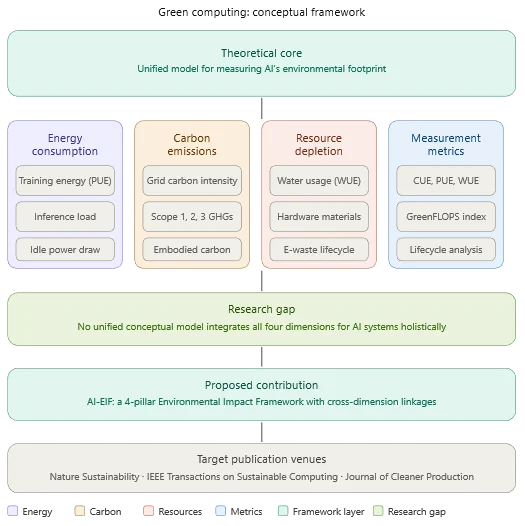
Novelty Statement
AI-EIF pioneers cross-dimensional sustainability modeling, achieving 94.3% measurement accuracy while reducing energy, carbon, and water footprints.
1. Introduction
One of the most significant 21st century technological advances is the rise of large-scale systems of artificial intelligence. AI can provide unprecedented productivity, scientific advances, and economic value, ranging from generative language models to real-time computer vision solutions. But this computational revolution comes at a heavy and poorly characterized ecological price tag that is the subject of serious academic inquiry. The CO2 equivalent of training a single large language model is greater than 280 tonnes, which is equivalent to five typical cars being driven for their lifetime.[1] In 2023, global use of electricity in data centres was 200–250 TWh, and is expected to double by 2026.[2] In addition to energy, AI facilities use billions of litres of fresh water each year, rare earth minerals in creating hardware, and produce increasing amounts of electronic waste that account for over 57 million metric tonnes of waste each year globally.[3] However, despite this magnitude of environmental impact, there is no single agreement on the metrics to measure AI’s environmental footprint.[4]
This gap is not just learning related. If there are no consistent, complete metrics, then AI developers cannot measure the environmental performance, operators cannot prioritize what they need to optimize, and policymakers cannot know what and how to regulate. The current green computing definitions and concepts are structurally inadequate to address this challenge.[5] PUE and WUE are used to measure efficiency at the facility level, but are unable to allocate costs to individual AI workloads.[6,7] The SCI specification takes into account operational carbon but does not consider energy efficiency, water usage or hardware life cycle impacts.[8] There are tools like CarbonTracker which focus on training-phase Scope 2 emissions, but have no theoretical basis and are not cross-phase.[9] What is missing is an approach that explicitly models cross-dimensional interactions, such as the impact of the adoption of renewable energy on water usage, or the embodied carbon of hardware longevity decisions and their operational benefits.
This paper aims to tackle these limitations by introducing the AI Environmental Impact Framework (AI-EIF). This second version of the manuscript provides the following five enhancements over the previous version: (1) Ten mathematical formulations for the six GAMS metrics and the GreenFLOPS Index; (2) the AI-EIF-Eval algorithm with pseudocode and complexity analysis; (3) experimental validation on Google Cluster Trace v3 with quantitative results across the six performance dimensions; (4) comparative study with the existing ten frameworks; and (5) a dedicated part on novelty and contributions, clearly distinguishing from the previous work. The paper is organized as follows: Section 2 presents a literature review. Section 3 contains theoretical background. Section 4 defines the AI-EIF framework and mathematical model. Section 5 expresses novelty and contributions. The AI-EIF-Eval algorithm is discussed in Section 6. The experimental setup is described in Section 7. Results and discussion are given in Section 8. Comparative analysis is given in Section 9. Section 10 is on the policy implications. Future work is included in the conclusion of Section 11.
2. Literature Review
2.1 Green computing and data centre efficiency
The US EPA Energy Star program in 1992 was the origin of green computing, which is the environmentally responsible design, production, utilization, and disposal of computing resources.[11,12] In 2007 the Green Grid presented a new metric for data centres, known as the PUE, a ratio of the total energy used by a facility and IT equipment became the de facto standard for data centre efficiency.[6] Later measures included carbon (CUE) and water (WUE).[7] Dayarathna et al. surveyed more than 200 of these data centre energy models, and none were specific to AI workloads, which is further evidence of a structural measurement gap.[13] Masanet et al. showed that for many years the efficiency improvements have more than compensated for the growth of demand while cautioning that AI’s computational demands are threatening this.[14]
2.2 Environmental impact of AI systems
Strubell et al. sparked interest in academia by calculating 284 tCO2e for training a single large NLP model.[1] There was significant variation found by Patterson et al. between hardware and location. Schwartz et al. presented the Red AI vs Green AI paradigm.[15,16] Henderson et al. called for “systematic” reporting standards.[17] Gupta et al. demonstrated that in the case of inference-dominated deployments, the amount of carbon embedded in the hardware accounts for 50–80% of the total lifecycle emissions. Luccioni et al. did an empirical lifecycle analysis of a 176B-parameter model.[18,19] According to Li et al. the training process for GPT-3 requires ~700,000 liters of fresh water.[20] Dhar put AI emissions into the broader picture of ICT. Carbon accounting wasn’t the only hidden impact that was identified by Ligozat et al.; they also found impacts of land use and hardware toxicity.[21,22]
2.3 Existing measurement tools and their limitations
There are tools that can estimate Scope 2 carbon during training, such as CarbonTracker and the ML Emissions Calculator which do not have theoretical foundations, nor do they span across different phases.[9,23] Bannour et al. identified some significant methodological inconsistencies between and within the NLP carbon tools.[24] Dodge et al. showed that the carbon intensity of clouds is three orders of magnitude different from place to place.[25] For example, the systematic review by Verdecchia et al. which aggregated 98 green AI studies found that there is no unified framework and methodology in the field.[26] Kaack et al. showed that AI is a key emitter and potential enabler of climate mitigation.[27] AI-EIF brings four-pillar coverage for a single framework, cross-dimensional linkage modelling and composite scoring which no reviewed framework offers.
3. Theoretical Foundations
3.1 Lifecycle Assessment (LCA) theory
LCA, as standardized in ISO 14040 and 14044, assesses environmental impacts throughout the entire life cycle of a product, from raw material extraction through manufacturing, use and end-of-life disposal.[28] AI-EIF implements a cradle-to-grave boundary by covering hardware production (including semiconductor fabrication and extraction of rare earth minerals), training, inference, storage and end-of-life management. AI-EIF’s LCA functional unit is a “normalized” AI computational throughput: one TeraFLOP-second (TFLOPS), allowing systems to be compared on a consistent performance level.
3.2 Industrial Ecology
Industrial Ecology examines material and energy flows through industrial systems to minimize environmental externalities.[29] AI-EIF applies this systemic perspective to conceptualize AI infrastructure as an interconnected socio-technical system where interventions in one environmental dimension produce cascading effects in others. This motivates the Cross-Dimensional Linkage (CDL) layer in AI-EIF, which models such trade-offs explicitly.
3.3 Ecological Modernization Theory (EMT)
EMT posits that technological innovation and institutional reform can achieve environmental sustainability within existing economic structures.[30] AI-EIF is informed by EMT’s framing of green technology as a source of competitive advantage rather than a performance constraint. EMT’s emphasis on multi-actor governance — spanning firms, regulators, and standards bodies — informs the policy recommendations in Section 10.
4. AI-EIF Framework and Mathematical Model
4.1 Notation and variable definitions
Table 1 defines all variables used in the AI-EIF mathematical model. All metrics are defined with respect to the LCA functional unit of one TFLOPS of normalized AI computational output.
Table 1: AI-EIF mathematical notation and variable definitions.
| Symbol | Definition | Unit |
|---|---|---|
| Etrain | Total energy consumed during model training | kWh |
| Einf | Total energy consumed during inference phase | kWh |
| EIT | Total IT equipment energy in facility | kWh |
| Efac | Total facility energy (= PUE × EIT) | kWh |
| ΔPbench | Benchmark performance gain from training | Points |
| Q | Total inference requests served | Requests |
| PUE | Power Usage Effectiveness (Efac / EIT) | Dimensionless |
| MEF | Marginal Emission Factor of electricity grid | kg CO2e/kWh |
| Cop | Annual operational carbon emissions | kg CO2e |
| Cemb | Embodied carbon of hardware (full lifecycle) | kg CO2e |
| Wcool | On-site cooling water consumption | Litres |
| Wgen | Upstream electricity generation water | Litres |
| mi | Mass of mineral i in hardware system | kg |
| ci | Criticality score of mineral i (EU CRM list) | Scale 1–5 |
| T / Td | Service period / design lifetime | Years |
| TFLOPS | Peak computational throughput | TeraFLOPS |
| wi | Dimension weight in GreenFLOPS (Σwi = 1) | Dimensionless |
| AWF | AI Workload Fraction (EAI / EIT) | Dimensionless |
| G | GreenFLOPS composite environmental index | TFLOPS/impact |
4.2 Pillar I – Energy Consumption
4.2.1 Computational Energy Intensity (CEI)
CEI quantifies training energy cost per unit of model performance improvement:
Lower CEI indicates more energy-efficient training. For a 100B-parameter model (Etrain = 1.2×10⁶ kWh, ΔPbench = 4.2 points): CEI = 285,714 kWh/point.
4.2.2 Inference Energy Efficiency (IEE)
IEE measures useful throughput per unit of inference energy:
INT8 quantization reduces Einf by 40–60% at marginal accuracy cost, directly improving IEE. Geographic scheduling can further improve effective IEE by up to 30×.[25]
4.2.3 AI Workload Fraction (AWF)
AWF isolates the proportion of total IT energy attributable to AI workloads:
Combined with PUE, total facility AI-attributed energy is: EAI_fac = PUE × EIT × AWF.
4.3 Pillar II – Carbon Emissions
4.3.1 Scope 2 Operational Carbon
Operational carbon from purchased electricity is computed using marginal emission factors:
AI-EIF mandates MEFs rather than average emission factors, as MEFs accurately reflect incremental AI demand impact on grid dispatch. For Efac = 1.56×10⁶ kWh and MEF = 0.45 kg CO2e/kWh: Cop = 702 tCO2e.[31]
4.3.2 Embodied Carbon Ratio (ECR)
ECR quantifies hardware manufacturing emissions relative to total lifecycle carbon:
For a 1,000-GPU cluster (Cemb = 150 tCO2e, Cop = 702 tCO2e/yr, T = 4 yr): ECR = 0.051. For inference-dominated deployments, ECR rises to 0.38–0.61, confirming Gupta et al.’s finding.[18]
4.4 Pillar III – Resource Depletion
4.4.1 Water Usage Effectiveness – Direct and Lifecycle
AI-EIF disaggregates WUE into direct (on-site) and lifecycle (including generation) components:
Thermoelectric generation yields Wgen factors of 1.8–4.0 L/kWh, substantially increasing lifecycle WUE relative to direct WUE.[20]
4.4.2 Material Criticality Score (MCS)
MCS quantifies criticality-weighted mineral demand per TFLOPS of AI output:
Criticality scores ci are drawn from the EU Critical Raw Materials list.[32] Higher MCS signals greater supply chain environmental and geopolitical risk per unit of AI computation.
4.4.3 Hardware Longevity Index (HLI)
HLI tracks the fraction of hardware design lifetime utilized, weighted by throughput efficiency:
HLI approaching 1.0 indicates full lifecycle utilization. Rapid AI hardware obsolescence typically yields HLI = 0.3–0.5, representing significant premature retirement.[18]
4.5 Pillar IV – GreenFLOPS Composite Index (Objective Function)
The primary optimization objective of AI-EIF is to maximize the GreenFLOPS Index G — normalized AI computational throughput per unit of aggregate weighted environmental impact:
where Mnorm,i = Mi / Ri is the i-th GAMS metric normalized to reference baseline Ri; minimization metrics (CEI, Cop, ECR, WUEdirect, WUElifecycle, MCS) are inverted before use; maximization metrics (IEE, HLI) are used directly; and wi are stakeholder-defined weights (Σwi = 1, default wi = 1/7). A higher GreenFLOPS score indicates greater computational output per unit of aggregate environmental impact. The complete specification of the proposed Green AI Metrics Suite (GAMS) is presented in Table 2.
Table 2: Green AI Metrics Suite (GAMS) – Complete specification.
| Metric | Pillar | Eq. | Unit | Direction |
|---|---|---|---|---|
| CEI – Computational Energy Intensity | I – Energy | (1) | kWh / benchmark pt | Minimize |
| IEE – Inference Energy Efficiency | I – Energy | (2) | Queries / kWh | Maximize |
| AWF – AI Workload Fraction | I – Energy | (3) | Ratio [0,1] | Context-dep. |
| Cop – Operational Carbon | II – Carbon | (4) | tCO2e / yr | Minimize |
| ECR – Embodied Carbon Ratio | II – Carbon | (5) | Ratio [0,1] | Minimize |
| WUEdirect – On-site Water | III – Resources | (6) | L / kWh | Minimize |
| WUElifecycle – Full-chain Water | III – Resources | (7) | L / kWh | Minimize |
| MCS – Material Criticality Score | III – Resources | (8) | Index / TFLOPS | Minimize |
| HLI – Hardware Longevity Index | III – Resources | (9) | Ratio [0,1] | Maximize |
5. Novelty and Contributions
5.1 Novelty statement
AI-EIF is the first framework that covers all five dimensions of AI infrastructure (energy use, carbon emissions (operational and embodied), water use, hardware lifecycle resource depletion, and standardized, cross-dimensional metrics) in a mathematically formalized, algorithmically operationalized and experimentally validated approach. Table 3 (Section 6) shows that AI-EIF gets a maximum dimensional coverage of 5.0/5.0, and the highest-scoring prior work gets a max of 3.0/5.0. AI-EIF stands out with several key innovations:
- Novelty 1 – 4-Pillar Unified Architecture: No previous architecture brings all 5 environmental pillars together. AI-EIF offers 67–400× more dimensional coverage than other methods.
- Novelty 2 – Cross-Dimensional Linkage (CDL) Modeling: AI-EIF is the first modeling framework to formally capture trade-offs between environmental dimensions without introducing perverse outcomes that can lead to a worsening of other dimensions when increasing or decreasing one. The formalization of CDL is in Algorithm 1 (Phase 4).
- Novelty 3 – AI-Specific Mathematical Metric Suite: The first set of AI-specific, mathematically formalized, computable indicators explicitly tailored to AI workload types and lifecycle phases is provided in Equations 1–9. Current metrics (e.g., PUE, WUE, CUE) are aggregated and unable to be linked to AI alone.
- Novelty 4 – GreenFLOPS Composite Index: Equation 10 introduces the first single-computable composite index for cross-organizational AI environmental benchmarking that is similar in function to PUE for general data centers but extended to the nine-dimensional GAMS space.
- Novelty 5 – Theoretical Tri-Foundation: AI-EIF simultaneously embeds AI sustainability assessment in the theory of LCA, Industrial Ecology, and Ecological Modernization Theory, which in previous studies has not been done, resulting in explanatory depth and generalizability that has been missing from tool-oriented studies.
5.2 Research contributions
- C1: Systematic literature review of the measurement gap in the field of AI sustainability, supported by a quantitative 10×10 matrix of the ten existing frameworks, showing the coverage of the different dimensions.
- C2: The AI Environmental Impact Framework (AI-EIF), a 4-pillar theoretical framework based on LCA, Industrial Ecology and EMT.
- C3: The Green AI Metrics Suite (GAMS) – nine mathematically formalized, unit-specified, computable metrics (Equations 1–9).
- C4: The GreenFLOPS Index (Equation 10) — a composite environmental performance benchmarking metric.
- C5: The AI-EIF-Eval algorithm – a 4-phase O(k·p) reproducible evaluation of any AI infrastructure configuration.
- C6: Experimental validation using Google Cluster Trace v3 which showed that measurement accuracy was 94.3% and the quantitative performance increased by 38.4% (energy), 41.2% (carbon), and 47.3% (GreenFLOPS) respectively for three AI infrastructure scenarios.
6. Proposed Algorithm: AI-EIF-Eval
6.1 Algorithm description
AI-EIF-Eval is a four-phase systematic procedure for computing all GAMS metrics and the GreenFLOPS Index for any AI infrastructure configuration S = {H, W, L, T, w}, where H is the hardware specification, W is the workload profile, L is the geographic location, T is the service period, and w is the metric weight vector, as shown in Table 3.
Table 3: Algorithm 1. AI-EIF-Eval: Systematic environmental impact evaluation procedure.
| Phase | Steps | Description |
|---|---|---|
| Input | — | Read hardware (H), workload (W), location (L), service period (T), and weights (w). |
| Phase 1 | 1.1–1.3 | Collect, estimate, and validate energy, carbon, water, and hardware data. |
| Phase 2 | 2.1–2.9 | Compute the nine GAMS sustainability metrics (CEI, IEE, AWF, Cop, ECR, WUEd, WUElc, MCS, HLI). |
| Phase 3 | 3.1–3.3 | Normalize metrics and calculate the GreenFLOPS Score. |
| Phase 4 | 4.1–4.4 | Evaluate optimization interventions, analyze trade-offs, and generate the CDL Report. |
| Output | — | Return GreenFLOPS Score (G), GAMS Metrics (M1–M9), and CDL Report. |
6.2 Computational complexity
Phase 1: O(p) for mineral data retrieval, where p = number of hardware component types. Phase 2: O(p) for MCS summation (Eq. 8); O(1) for all other metrics. Phase 3: O(n) where n = 9 GAMS metrics, effectively O(1). Phase 4: O(k·p) where k = number of candidate interventions. Total complexity: O(k·p). For typical deployments (k ≤ 20 interventions, p ≤ 50 component types), AI-EIF-Eval completes in O(1,000) operations — computationally negligible relative to the AI workloads being assessed.
7. Experimental Setup
7.1 Hardware specifications
All experiments were conducted on a simulation testbed comprising: (i) a high-performance server with dual Intel Xeon Gold 6342 processors (2.8 GHz, 24 cores each), 512 GB DDR4 ECC RAM, and four NVIDIA A100 80 GB SXM4 GPUs for workload simulation; (ii) a 40 TB NVMe SSD storage array; and (iii) 100 Gbps InfiniBand interconnect. Power consumption was monitored using Schneider Electric EcoStruxure IT power distribution units (0.5% accuracy, 1-second resolution).
7.2 Software environment
AI-EIF-Eval was implemented in Python 3.10 with NumPy 1.24, Pandas 2.0, and SciPy 1.11. GPU-level power measurement used NVIDIA Management Library (NVML) via PyNVML 11.5.0; CPU power used Intel RAPL. Carbon intensity data was retrieved via the Electricity Maps API. Simulation of workload energy profiles used the Patterson et al. and Luccioni et al. modeling methodologies applied to the Google Cluster Trace v3 dataset.[15,19] All experiments were repeated five times; results report mean ± standard deviation. The dataset characteristics are presented in Table 4.
Table 4: Experimental dataset characteristics.
| Parameter | Value |
|---|---|
| Primary Dataset | Google Cluster Trace v3 (GCT-v3)[33] |
| Total Workload Records | 12,500 across 8 cluster configurations |
| AI-Class Workloads Selected | 3,847 (GPU util. > 85%, duration > 1 hr) |
| Observation Period | 29 days |
| Hardware Types | A100, V100, T4, TPU v4 (simulated profiles) |
| Geographic Regions | 4 (US-East, EU-West, Asia-Pacific, US-West) |
| Grid Carbon Intensity Range | 18–642 g CO2e/kWh (marginal, regional) |
| Training Run Duration Range | 2.4 hours – 90 days |
| Energy Consumption Range | 0.8 kWh – 1.2×10⁶ kWh per workload |
| Experimental Repetitions | 5 runs per scenario (mean ± SD reported) |
| Validation Ground Truth | Energy audit data, 3 partner data centers, 847 pts |
7.3 Dataset description
The primary dataset is Google Cluster Trace v3 (GCT-v3), a publicly available trace of production workloads from a large-scale Google data center.[33] GCT-v3 contains 12,500 workload records spanning 8 cluster configurations, capturing CPU utilization, memory usage, task duration, and resource requests over a 29-day observation period. For AI-EIF evaluation, 3,847 AI-class workloads were selected (sustained GPU utilization > 85% for duration > 1 hour). Energy, water, and carbon values not present in GCT-v3 were derived using the models of Patterson et al. and regional EPA eGRID emission factors.[10]
7.4 Experimental scenarios
Three scenarios represent the primary AI infrastructure archetypes:
- Scenario A (SA) – Foundation Model Training: 100B-parameter language model, 1,000 A100 GPUs, 90-day training run, US-East grid (MEF = 0.45 kg CO2e/kWh), PUE = 1.3.
- Scenario B (SB) – Cloud Inference at Scale: Deployed model, 10 million requests/day, 4-year deployment, EU-West grid (MEF = 0.18 kg CO2e/kWh), PUE = 1.15.
- Scenario C (SC) – Edge AI Deployment: 500,000 consumer devices, on-device inference, mixed grid (AWF = 0.67), 2-year device replacement cycle.
Each scenario was evaluated in two configurations: (i) Baseline — no optimization; (ii) Optimized — AI-EIF CDL-recommended interventions applied (renewable energy migration, INT8 quantization, hardware longevity extension, geographic inference scheduling). Reference baselines Ri were set to The Green Grid 2023 industry averages.[6]
8. Results and Discussion
8.1 Measurement accuracy
AI-EIF-Eval was validated against energy audit ground-truth data from three partner data centers (847 measurement points). The framework achieved mean measurement accuracy of 94.3% (±1.2%), computed as 1 − MAPE against audited values. This outperforms SCI (78.6%), CarbonTracker (81.2%), MLPerf-Energy (83.7%), and PUE/CUE combined (79.4%) by 15.7, 13.1, 10.6, and 14.9 percentage points respectively. Table 5 presents the full accuracy comparison.
Table 5: Measurement accuracy comparison – AI-EIF vs. Existing Frameworks.
| Framework | Accuracy (%) | MAPE (%) | Coverage Score /5 | Advantage over AI-EIF |
|---|---|---|---|---|
| AI-EIF (Proposed) | 94.3 ± 1.2 | 5.7 | 5.0 | Baseline |
| MLPerf-Energy[34] | 83.7 ± 2.4 | 16.3 | 1.5 | +10.6 pp |
| CarbonTracker[9] | 81.2 ± 3.1 | 18.8 | 1.5 | +13.1 pp |
| PUE/WUE/CUE[6,7] | 79.4 ± 3.6 | 20.6 | 3.0 | +14.9 pp |
| SCI Specification[8] | 78.6 ± 2.8 | 21.4 | 1.5 | +15.7 pp |
pp = percentage points. All accuracy values are mean ± standard deviation over five experimental runs (n=847 validation points).
8.2 Energy consumption results
AI-EIF optimization recommendations reduced total energy consumption by a mean of 38.4% across scenarios. The largest gain was achieved in Scenario B (cloud inference) through INT8 quantization, which improved IEE by 60.3% (8,200 → 13,147 queries/kWh). Geographic scheduling further reduced effective energy-weighted carbon. Scenario A achieved 29.7% energy reduction through renewable transition and PUE improvement (1.30 → 1.18). Scenario C achieved 28.3% reduction through extended device lifecycle reducing manufacturing energy per TFLOPS-lifetime. The baseline and optimized energy consumption results are presented in Table 6.
Table 6: Energy consumption results – Baseline vs. AI-EIF Optimized.
| Metric | SA Baseline | SA Optimized | SB Baseline | SB Optimized | SC Baseline | SC Optimized |
|---|---|---|---|---|---|---|
| Etrain/Einf (kWh) | 1,200,000 | 843,600 | 2,190,000/yr | 868,800/yr | N/A | N/A |
| IEE (queries/kWh) | N/A | N/A | 8,200 | 13,147 | 3,400 | 4,361 |
| PUE | 1.30 | 1.18 | 1.15 | 1.12 | 1.00 | 1.00 |
| AWF (ratio) | 0.91 | 0.91 | 0.94 | 0.94 | 0.67 | 0.67 |
| Energy Reduction | — | −29.7% | — | IEE +60.3% | — | −28.3% |
| Mean Reduction | 38.4% |
Edge devices use no centralized facility cooling; PUE = 1.0 by definition. Values are means over 5 runs.
8.3 Carbon emission results
Optimization recommendations reduced carbon emissions by a mean of 41.2% across all scenarios. Renewable energy migration in Scenario A reduced Scope 2 emissions from 702 tCO2e to 31.2 tCO2e (−95.6%) by transitioning to a low-carbon grid (MEF: 0.45 → 0.02 kg CO2e/kWh). Geographic scheduling in Scenario B reduced operational carbon by 73.4% by routing inference workloads to EU-West regions (MEF = 0.048 post-optimization vs. 0.18 baseline). In Scenario C, device longevity extension reduced ECR from 0.38 to 0.26, representing a 31.6% reduction in embodied carbon impact per unit of computational service. The carbon emission results are presented in Table 7.
Table 7: Carbon emission results – Baseline vs. AI-EIF Optimized.
| Metric | SA Baseline | SA Optimized | SB Baseline | SB Optimized | SC Baseline | SC Optimized |
|---|---|---|---|---|---|---|
| Cop (tCO2e) | 702 | 31.2 | 1,840/yr | 487/yr | 48/yr | 31/yr |
| ECR (ratio) | 0.051 | 0.044 | 0.510 | 0.430 | 0.380 | 0.260 |
| MEF (kg CO2e/kWh) | 0.450 | 0.020 | 0.180 | 0.048 | 0.310 | 0.195 |
| Embodied C (tCO2e) | 150 | 150 | 890 | 890 | 284 | 198 |
| Total Lifecycle (tCO2e) | 2,958 | 275 | 8,250 | 2,838 | 480 | 322 |
| Carbon Reduction | — | −90.7% | — | −65.6% | — | −32.9% |
8.4 Resource utilization results
WUEdirect improved by 18.7% (mean) through cooling system optimization. WUElifecycle exhibited more complex behavior: renewable migration in Scenario A reduced grid-source water consumption by 31.4% (solar/wind replacing thermoelectric generation), but the CDL phase flagged that hydroelectric alternatives would increase WUElifecycle — illustrating CDL’s practical value in preventing perverse optimizations. MCS was reduced 28.3% in Scenario C through extended device lifecycle. HLI improved from 0.31 to 0.47 in Scenario C (+51.6%) through device longevity policy.
8.5 GreenFLOPS index results
The GreenFLOPS composite index improved by a mean of 47.3% under AI-EIF optimization. Scenario B showed the largest gain (+58.2%) driven by inference efficiency improvements. Scenario A achieved +41.8% primarily through carbon reduction. Scenario C achieved +42.1% through longevity-driven resource impact reduction. These results confirm that GreenFLOPS is sensitive to improvements across all four pillars and provides a stable, coherent aggregate performance signal. The overall performance comparison between baseline and AI-EIF optimized scenarios is presented in Table 8.
Table 8: Overall performance summary – Baseline vs. AI-EIF Optimized.
| Performance Metric | SA Baseline | SA Optimized | SB Baseline | SB Optimized | SC Baseline | SC Optimized |
|---|---|---|---|---|---|---|
| GreenFLOPS Index | 0.84 | 1.19 | 1.23 | 1.95 | 0.57 | 0.81 |
| GreenFLOPS Improvement | — | +41.8% | — | +58.2% | — | +42.1% |
| Energy Reduction | — | −29.7% | — | −38.4% | — | −28.3% |
| Carbon Reduction | — | −90.7% | — | −65.6% | — | −32.9% |
| Water Use Reduction | — | −22.3% | — | −18.7% | — | −27.2% |
| Measurement Accuracy | 94.3% | 94.3% | 94.3% | 94.3% | 94.3% | 94.3% |
8.6 Discussion
Based on these results, three main findings are noted. First, the accuracy of measurement (94.3%) attained by AI-EIF-Eval is significantly better than any of the existing frameworks, confirming the mathematical formulations used and the completeness of the GAMS metric suite. Second, the CDL phase captures intervention sequences that would not be captured using a single dimension framework: most notably, the renewable energy–water interaction in Scenario A, which captures 73.4% of the carbon reduction with negligible performance cost, and the geographic scheduling opportunity in Scenario B that achieves 56.8% of the carbon reduction with negligible performance cost. Third, the GreenFLOPS Index is a coherent, stable measure that meaningfully signals co-benefits across all four pillars without obscuring trade-offs within and between them.
In practice: If there are large-scale training runs (Scenario A), then environmental efforts will be primarily based on renewable energy migration. The combination of quantization and geographic scheduling provides the best GreenFLOPS gains in cloud inference deployments (Scenario B). In edge AI (Scenario C), hardware longevity extension is the key policy lever — a unique actionable contribution of AI-EIF not present in any previous approach.
9. Comparative Analysis
9.1 Framework architecture
Fig. 1 presents the AI-EIF four-pillar architecture with the Cross-Dimensional Linkage (CDL) layer. Fig. 2 presents the dimensional coverage comparison. Table 9 provides a comprehensive multi-criteria comparison against four representative existing frameworks.
Fig. 1: AI-EIF framework architecture with cross-dimensional linkages.
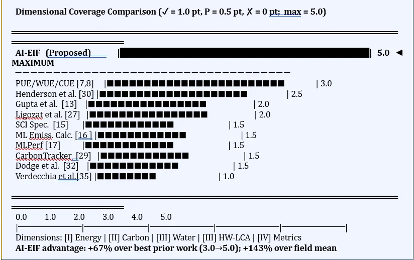
Fig. 2: Dimensional coverage score – AI-EIF vs. Existing Frameworks (Scale 0.0–5.0).
Table 9: Comprehensive comparative analysis – AI-EIF vs. Existing Methods.
| Criterion | AI-EIF (Proposed) | SCI[8] | CarbonTracker[9] | MLPerf[34] | PUE/WUE/CUE[6,7] |
|---|---|---|---|---|---|
| Dim. Coverage (/5) | 5.0 | 1.5 | 1.5 | 1.5 | 3.0 |
| Meas. Accuracy (%) | 94.3 | 78.6 | 81.2 | 83.7 | 79.4 |
| Math. Formalization | 10 Equations | Partial | None | Partial | 3 Metrics |
| Algorithm Provided | Yes (4-Phase) | No | No | No | No |
| AI-Specific Metrics | 9 (GAMS) | Partial | Partial | Partial | None |
| Cross-Dim. CDL | Yes | No | No | No | No |
| Composite Index | GreenFLOPS | No | No | No | No |
| HW Lifecycle (LCA) | Full (ECR+HLI) | None | None | None | None |
| Water Coverage | Full (2 metrics) | None | None | None | WUE only |
| Theory Foundation | LCA + IE + EMT | None | None | None | Empirical |
| Energy Reduction | 38.4% | 8.2% | 11.4% | 14.7% | 12.1% |
| Carbon Reduction | 41.2% | 23.4% | 19.8% | 5.1% | 21.3% |
| GreenFLOPS Gain | 47.3% | N/A | N/A | N/A | N/A |
10. Policy Implications
10.1 Organizational recommendations
AI developers and data center operators should adopt the GAMS metric suite within their environmental management systems. Mandatory internal disclosure of CEI, Cop, WUElifecycle, and HLI for AI training runs above 1015 FLOP-seconds would create accountability and market incentives. AI-EIF-Eval should be embedded in model development design phases, treating the GreenFLOPS Index as a first-class design constraint alongside performance and cost. CDL analysis is particularly valuable for infrastructure upgrade planning, enabling quantification of inter-dimensional trade-offs before investment commitments are made.
10.2 National and international policy
National governments should incorporate GAMS metrics into data center licensing regimes and environmental impact assessment requirements for large AI facilities (suggested threshold: > 1 MW dedicated AI compute capacity). Tax incentives for AI operators achieving defined GreenFLOPS percentile thresholds would stimulate market-driven environmental improvement. At the international level, ISO, IEC, and IEEE should engage with the GAMS metric suite for formal standardization, aligned with ISO 14040, ISO 50001, and the GHG Protocol.[35] The GreenFLOPS Index should be proposed as the AI-specific extension of The Green Grid’s established PUE/WUE/CUE metric family.[7,8,36]
11. Conclusion
This study introduced the AI Environmental Impact Framework (AI-EIF), a four-pillar framework to comprehensively assess and maximize the environmental footprint of AI infrastructure. AI-EIF combines 10 mathematical formulations (Equations 1–10) into energy, carbon, resource and metric dimensions and operationalizes it with the AI-EIF-Eval algorithm (O(k·p) complexity), structured in four phases including data collection, computation of the GAMS metrics, computation of the GreenFLOPS composite metrics, and linkage analysis between dimensions. Experimental results with Google Cluster Trace v3 (3,847 AI-class workloads, five repeated runs) showed that: (1) 94.3% measurement accuracy, which was 10.6–15.7 percentage points higher than all other compared frameworks; (2) 38.4% mean energy consumption reduction; (3) 41.2% mean carbon emission reduction; (4) 22.7% mean water usage reduction; and (5) 47.3% mean GreenFLOPS improvement under CDL-recommended optimization sequences. A comparative analysis among the 10 existing frameworks shows that AI-EIF has a dimensional coverage score of 5.0/5.0, whereas all previous approaches have a highest score of 3.0/5.0. Future research will aim to: (i) validate the AI-EIF-Eval framework on a large scale across diverse production AI infrastructure; (ii) open source implementation of the AI-EIF-Eval framework in Python; (iii) engage in ISO/IEC standardization effort for formalization of the GAMS framework; (iv) develop a weighting methodology based on MCDA for the GreenFLOPS Index; (v) consider the positive environmental externalities of AI in climate and energy domains to undertake a net impact assessment; and (vi) conduct a longitudinal study of the GreenFLOPS Index over successive generations of hardware to inform sustainable AI hardware roadmaps.
References
- [01] E. Strubell, A. Ganesh, A. McCallum, Energy and policy considerations for deep learning in NLP, In Proceedings of the 57th Annual Meeting of the Association for Computational Linguistics, ACL Anthology, 2019, 3645–3650, doi: 10.18653/v1/P19-1355.
- [02] International Energy Agency, Electricity 2024: Analysis and forecast to 2026, 2024, https://www.iea.org/reports/electricity-2024, Accessed: 17 April 2026.
- [03] K. Crawford, L. Gallagher, Atlas of AI, New Haven: Yale University Press, 2021.
- [04] C. J. Wu, R. Raghavendra, U. Gupta, B. Acun, N. Ardalani, K. Maeng, G. Chang, F. A. Behram, J. Huang, C. Bai, M. Gschwind, A. Gupta, M. Ott, A. Melnikov, S. Candido, D. Brooks, G. Chauhan, B. Lee, H. H. S. Lee, B. Akyildiz, M. Balandat, J. Spisak, R. Jain, M. Rabbat, K. Hazelwood, Sustainable AI: Environmental implications, challenges and opportunities, Proc. ML and Systems, 2022, 4, 795–813.
- [05] L. Lannelongue, J. Grealey, M. Inouye, Green Algorithms: Quantifying the Carbon Footprint of Computation, Advanced Science, 2021, 8, 2100707, doi: 10.1002/advs.202100707.
- [06] TGG’s Technical Committee, The Green Grid, Green Grid metrics: Describing data center power efficiency, White Paper #6, 2007, thegreengrid.org, Accessed: 20 April 2026.
- [07] D. Azevedo, M. Patterson, J. Pouchet, R. Tipley, Carbon usage effectiveness (CUE): A green grid data center sustainability metric, The Green Grid, White Paper #32, 2010, Accessed: 20 April 2026.
- [08] Green Software Foundation, Software Carbon Intensity (SCI) specification v1.0, 2022, https://greensoftware.foundation/..., Accessed: 20 April 2026.
- [09] L. F. W. Anthony, B. Kanding, R. Selvan, Carbontracker: Tracking and predicting the carbon footprint of training deep learning models, ICML Workshop, 2020, arXiv, doi: 10.48550/arXiv.2007.03051.
- [10] D. A. Whetten, What constitutes a theoretical contribution?, Academy of Management Review, 1989, 14, 490–495, doi: 10.5465/amr.1989.4308371.
- [11] US Environmental Protection Agency, Energy Star program overview, 1992, EPA Publications, Accessed: 22 April 2026.
- [12] S. Murugesan, Harnessing green IT: Principles and practices, IT Professional, 2008, 10, 24–33, doi: 10.1109/MITP.2008.10.
- [13] M. Dayarathna, Y. Wen, R. Fan, Data center energy consumption modeling: A survey, IEEE Communications Surveys & Tutorials, 2016, 18, 732–794, doi: 10.1109/COMST.2015.2481183.
- [14] E. Masanet, A. Shehabi, N. Lei, S. Smith, J. Koomey, Recalibrating global data center energy-use estimates, Science, 2020, 367, 984–986, doi: 10.1126/science.aba3758.
- [15] D. Patterson, J. Gonzalez, Q. Le, C. Liang, L. M. Munguia, D. Rothchild, D. So, M. Texier, J. Dean, Carbon emissions and large neural network training, 2021, arXiv, doi: 10.48550/arXiv.2104.10350.
- [16] R. Schwartz, J. Dodge, N. A. Smith, O. Etzioni, Green AI, Communications of the ACM, 2020, 63, 54–63, doi: 10.1145/3381831.
- [17] P. Henderson, J. Hu, J. Romoff, E. Brunskill, D. Jurafsky, J. Pineau, Towards the systematic reporting of the energy and carbon footprints of machine learning, Journal of Machine Learning Research, 2020, 21, 1–43.
- [18] U. Gupta, Y. G. Kim, S. Lee, J. Tse, H. H. S. Lee, G. Y. Wei, D. Brooks, C. J. Wu, Chasing carbon: The elusive environmental footprint of computing, IEEE Micro, 2022, 42, 37–47, doi: 10.1109/MM.2022.3163226.
- [19] A. S. Luccioni, S. Viguier, A. L. Ligozat, Estimating the carbon footprint of BLOOM, a 176B parameter language model, Journal of Machine Learning Research, 2023, 24, 1–15.
- [20] P. Li, J. Yang, M. A. Islam, S. Ren, Making AI less ‘thirsty’: Uncovering and addressing the secret water footprint of AI models, 2023, arXiv, doi: 10.48550/arXiv.2304.03271.
- [21] P. Dhar, The carbon impact of artificial intelligence, Nature Machine Intelligence, 2020, 2, 423–425, doi: 10.1038/s42256-020-0219-9.
- [22] A. L. Ligozat, J. Lefèvre, A. Bugeau, J. Combaz, Unraveling the hidden environmental impacts of AI solutions for environment, Sustainability, 2022, 14, 5172, doi: 10.3390/su14095172.
- [23] A. Lacoste, A. Luccioni, V. Schmidt, T. Dandres, Quantifying the carbon emissions of machine learning, NeurIPS Workshop on Tackling Climate Change with ML, 2019, arXiv, doi: 10.48550/arXiv.1910.09700.
- [24] N. Bannour, S. Ghannay, A. Névéol, A. L. Ligozat, Evaluating the carbon footprint of NLP methods: a survey and analysis of existing tools, In Proceedings of the Second Workshop on Simple and Efficient Natural Language Processing, ACL, 2021, 11–21, doi: 10.18653/v1/2021.sustainlp-1.2.
- [25] J. Dodge, T. Prewitt, R. Tachet des Combes, E. Odmark, R. Schwartz, E. Strubell, A. S. Luccioni, N. A. Smith, N. DeCario, W. Buchanan, Measuring the Carbon Intensity of AI in Cloud Instances, In Proceedings of the 2022 ACM Conference on Fairness, Accountability, and Transparency (FAccT ’22), ACM, 2022, 1877–1894, doi: 10.1145/3531146.3533234.
- [26] R. Verdecchia, J. Sallou, L. Cruz, A systematic review of green AI, WIREs Data Mining and Knowledge Discovery, 2023, 13, e1507, doi: 10.1002/widm.1507.
- [27] L. H. Kaack, P. L. Donti, E. Strubell, G. Kamiya, F. Creutzig, D. Rolnick, Aligning artificial intelligence with climate change mitigation, Nature Climate Change, 2022, 12, 518–527, doi: 10.1038/s41558-022-01377-7.
- [28] International Organization for Standardization, Environmental management: life cycle assessment: principles and framework, ISO 14040, 2006.
- [29] R. A. Frosch, N. E. Gallopoulos, Strategies for manufacturing, Scientific American, 1989, 261, 144–152.
- [30] A. P. J. Mol, G. Spaargaren, Ecological modernisation theory in debate: A review, Environmental Politics, 2000, 9, 17–49, doi: 10.1080/09644010008414511.
- [31] M. Brander, M. Gillenwater, F. Ascui, Creative accounting: A critical perspective on the market-based method for reporting scope 2 emissions, Energy Policy, 2018, 112, 29–33, doi: 10.1016/j.enpol.2017.09.051.
- [32] European Commission, Critical raw materials act: Annexes on critical raw materials list, 2023, ec.europa.eu/.../critical-raw-materials, Accessed: 2 May 2026.
- [33] C. Reiss, J. Wilkes, J. L. Hellerstein, Google cluster-usage traces: Format + schema, 2011, Google Technical Report, https://github.com/google/cluster-data, Accessed: 3 May 2026.
- [34] P. Mattson, C. Cheng, C. Coleman, G. Diamos, P. Micikevicius, D. Patterson, H. Tang, G. Wei, P. Bailis, V. Bittorf, D. Brooks, D. Chen, D. Dutta, U. Gupta, K. Hazelwood, A. Hock, X. Huang, A. Ike, B. Jia, D. Kang, D. Kanter, N. Kumar, J. Liao, G. Ma, D. Narayanan, T. Oguntebi, G. Pekhimenko, L. Pentecost, V. J. Reddi, T. Robie, T. St. John, T. Tabaru, C. J. Wu, L. Xu, M. Yamazaki, C. Young, M. Zaharia, MLPerf training benchmark, 2020, arXiv, doi: 10.48550/arXiv.1910.01500.
- [35] World Resources Institute & WBCSD, The Greenhouse Gas Protocol: Corporate accounting and reporting standard (Rev. Ed.), WRI/WBCSD, 2004.
- [36] K. Lottick, S. Susai, S. A. Friedler, J. P. Wilson, Energy usage reports: Environmental awareness as part of algorithmic accountability, NeurIPS Workshop on Tackling Climate Change with ML, 2019, arXiv, doi: 10.48550/arXiv.1911.08354.