

 Open Access||Research Article
Fuzzy Logic-based PWM Control of a Three-Phase Synchronous Rectifier for Low-Speed Wind Energy Conversion
Ika Noer Syamsiana1 , Muhammad Akmal Nashiry1, Harrij Mukti Khristiana1, Arwin Datumaya Wahyudi Sumari2
1 Electrical Power Systems Study Program, Department of Electrical Engineering, State Polytechnic of Malang, Malang 65141, East Java, Indonesia
2 Office of Special High-Rank Officer, Indonesian Air Force Headquarters, Jakarta Timur, DKI Jakarta, 13870, Indonesia
Abstract
Low-speed wind energy conversion systems require an effective power-electronic interface to manage low and fluctuating generator voltages. In this study, a Mamdani fuzzy logic controller (FLC) for regulating the Pulse-Width Modulation (PWM) duty cycle of a three-phase synchronous Metal-Oxide-Semiconductor Field-Effect Transistor (MOSFET) rectifier intended for low-speed wind energy conversion is developed. The controller employs the voltage error and change in error as its inputs, an 5×3inference matrix comprising 15 rules, and duty-cycle correction as its output. The FLC was designed and evaluated in MATLAB/Simulink, while its circuit-level implementation, including an Arduino UNO model, three IR2110 gate drivers, MOSFET switching devices, and resistive and resistive–inductive loads, was verified in Proteus. The simulations investigated the effects of the duty cycle, input voltage, and load variations on the rectifier output. The maximum DC output remained close to the theoretical value of 64.8 V, with deviations below 2.5% across the evaluated duty cycle range. The output ripple increased from 1.4–2.2% at a 30% duty cycle to 8.2–9.8% at duty cycles of 50% and above. This behavior was associated with the absence of a series filter inductor in the investigated topology. At an AC input voltage of 48 V, the FLC regulated the output close to the 48 V reference. At an input of 36 V, the controller reached its maximum duty cycle limit because the selected reference exceeded the achievable conversion range. The results demonstrate the simulation-level feasibility of the proposed FLC and identify the source voltage, filtering configuration, and rectifier topology as the principal constraints on voltage regulation.
Keywords
Graphical Abstract
Novelty Statement
The novelty of this study lies in the direct application of a Mamdani fuzzy logic controller to PWM duty-cycle regulation in a three-phase synchronous MOSFET rectifier intended for low-speed wind energy conversion. The study integrates controller-level analysis in MATLAB/Simulink with circuit-level verification in Proteus, incorporating virtual models of the Arduino UNO, IR2110 gate drivers, MOSFET switching stage, and resistive and resistive–inductive loads. It further characterizes a ripple-plateau behavior in the simulated inductor-less rectifier configuration and distinguishes controller saturation from the physical voltage-conversion constraints imposed by the source and converter topology.
1. Introduction
Indonesia’s installed power generation capacity reached 73,461 MW in 2023, approximately 53.7% (39,413 MW) of which still relies on fossil-fuelled steam power plants, raising well-known environmental and economic concerns.[1] Under the 2025–2034 Electricity Supply Business Plan (ESBP), the government targets 69.5 GW of additional capacity, 61% of which (42.6 GW) is planned to come from new and renewable energy, with wind power contributing approximately 7.2 GW of that share.[2] Wind energy is widely regarded as one of the most technically mature and scalable renewable resources; however, despite a theoretical national potential exceeding 150 GW, Indonesia’s installed wind capacity remains only a small fraction of that figure, reflecting how far deployment still lags behind resource availability.[3] Much of this shortfall traces to wind speed characteristics: recent utility-scale site assessments across coastal and inland regions in Indonesia continue to find viable locations only at moderate hub heights and capacity factors, underscoring that even the country’s better wind corridors do not resemble the strong, sustained wind regimes assumed by conventional turbine design.[4] The average wind speeds across most of Indonesia, including Malang (up to approximately 4.5 m/s) and the northern coast of Cirebon (2.7–3.9 m/s), fall in the low-to-moderate category, a condition shared by many low-wind developing country sites where wind energy conversion systems (WECSs) must be engineered to extract usable power despite fluctuating, low-amplitude generator outputs. [5-7] Under these conditions, both the maximum-power-point-tracking strategy and the downstream power-conditioning stage must be designed explicitly around low and variable inputs rather than assumed.[8,9] A low-speed wind power generation design is therefore required to exploit this resource, but the resulting generator output is inherently unstable in both amplitude and frequency and requires power conditioning before it can supply a load or a battery bank.[10]
In a wind energy conversion system, the chain from the turbine to usable power runs through the generator, the rectifier, and the DC link or load: the turbine converts wind kinetic energy into mechanical rotation; the generator converts that rotation into three-phase AC; and the rectifier converts the AC into a DC quantity that can be regulated, stored, or inverted.[6,10] The rectifier stage is therefore not a passive afterthought but an active interface whose behavior determines how much of the fluctuating generator output actually becomes usable power, a point reinforced by recent studies that pair permanent-magnet synchronous generators with dedicated rectifier or DC-DC stages specifically to hold the output within a usable voltage band despite wind speed variation.[11] An uncontrolled diode rectifier is simple, inexpensive, and reliable, but it offers no mechanism to regulate or shape its output; its voltage and current are dictated entirely by the generator and load conditions.[12] A synchronous rectifier built from actively switched MOSFETs, by contrast, adds a controllable degree of freedom: by adjusting the PWM duty cycle applied to the switching bridge, it becomes possible to influence the DC-link voltage, the output ripple, the conduction losses, and the response to input or load disturbances.[13,14] Realizing this controllable degree of freedom in practice still depends on component-level choices that are easy to overlook in a control-oriented design: the switching devices, the printed circuit board that interconnects them, the gate-driver stage that delivers the PWM command to each MOSFET, and the microcontroller that generates it.[15-18] This flexibility does not mean that the output voltage can be raised without limit; the achievable range is still bounded by the AC source amplitude, the rectifier topology, and the energy-storage elements present at the output, so duty-cycle control must be understood as a way of shaping the output within these physical limits rather than overriding them.[7,19]
Because a low-speed wind turbine produces a generator voltage that varies with the wind speed and because the load connected to the rectifier can itself change over time, the PWM rectifier must address two independent sources of disturbance at once, a challenge widely noted in recent low-voltage-ride-through and maximum-power-point-tracking reviews of wind energy conversion systems.[8,9] An open-loop duty-cycle setting cannot correct for either disturbance: it can reproduce only the output of the fixed switching pattern produced for the AC input and load present at that moment.[20] Widening the duty cycle also has side effects beyond simply shifting the average output voltage; in a topology without a series filter inductor, it changes how long the output capacitor is left to discharge between switching pulses, which in turn affects the ripple content of the DC output.[14,19,21] Similarly, a voltage setpoint that exceeds what the present AC input can theoretically support will drive any duty-cycle controller toward saturation regardless of how well that controller is designed, a constraint that surfaces repeatedly in converter-level studies of PMSG-based wind systems operating away from their rated voltage.[6,7] Because the switching stage itself is modeled on a low-cost, resource-constrained platform, an 8-bit microcontroller together with Proteus-modeled gate-driver and MOSFET blocks, the controller must also remain simple enough to execute reliably within a fixed control-loop period, a practical constraint reported in comparable Arduino- and Proteus-based embedded power-control simulations.[22,23] These interaction effects, such as wind-driven input variation, load variation, ripple sensitivity to the duty cycle, and setpoint feasibility, are practical motivations for moving from an open-loop PWM pattern to a closed-loop controller that continuously senses the output and corrects the duty cycle in response.
Rectifier and converter control has traditionally relied on fixed-gain proportional-integral (PI) controllers, and for good reason, a PI loop is simple to implement, well understood, and adequate when the plant behaves close to linear around a single operating point.[14] The difficulty is that a three-phase PWM rectifier is not such a plant. Its behavior changes with the duty cycle, input voltage, and load, and it includes inherently nonlinear and switched dynamics that a fixed-gain PI controller was never tuned to cover.[14,20,23] Under these conditions, a PI controller that performs well at one operating point may respond poorly, oscillate, or require retuning at another; recent hardware and simulation comparisons on DC-DC and rectifier-adjacent converters consistently report that a fuzzy controller reaches its target faster and with less overshoot than a comparably tuned PID or PI loop under the same disturbance.[23-25] Fuzzy logic control (FLC) offers an alternative that does not require a precise mathematical model of the plant; instead, it encodes heuristic, human-like decision rules that map an observed error and its rate of change directly onto a corrective action, an approach that has also proven implementable on resource-limited embedded controllers similar to the one used in this study.[7,22,26] These characteristics make fuzzy logic a suitable candidate for regulating the PWM duty cycle under nonlinear and varying operating conditions; this does not, on its own, establish that a fuzzy controller outperforms a well-tuned PI controller in this particular application, a comparison that lies outside the scope of the present study.[8]
Fuzzy-based control of PWM rectifiers and wind energy conversion systems has been explored in recent years. Direct power control (DPC) combined with fuzzy switching-state selection has been shown to reduce current total harmonic distortion to as low as 0.31%; an adaptive fuzzy DPC-SVM scheme for hybrid PV/wind microgrids has reported ripple reductions of up to 80% relative to a conventional PI controller, and a hybrid fuzzy MPPT strategy has been applied to PMSG-based wind conversion connected to a smart grid.[27-29] At the rectifier level specifically, a type-3 fuzzy logic controller has recently been proposed for the DC-bus voltage regulation of a three-phase PWM rectifier, reporting shorter settling times and lower overshoot than both a conventional PI controller and a type-1 fuzzy controller under load transients and regenerative operation.[14] A direct comparison between an optimized PI controller and a Mamdani-type FLC for a grid-connected wind turbine likewise reported improvements in settling time and steady-state error under fault conditions, whereas a similar comparison for a DC–DC boost converter revealed that the fuzzy controller reduced the rise time and overshoot relative to a PID controller at the cost of a small increase in steady-state error.[23-25] Nonfuzzy approaches, such as a Vienna-rectifier vector control strategy validated on a PMSG test bench under a variable wind profile and a dq-transform double-loop controller with a stepped voltage-setting strategy, have also achieved fast, low-overshoot regulation, and broader reviews of WECS power-converter control continue to catalog MPPT, DPC, and intelligent control variants without converging on a single preferred approach for low-speed, low-cost installations.[6,7,8,20] These studies are validated primarily in MATLAB/Simulink, where a physical rectifier is used at all, target grid-connected or DPC/MPPT-based control objectives; comparatively little work applies a Mamdani FLC directly to the duty-cycle regulation of a stand-alone, low-speed wind rectifier with an explicit, block-by-block account of the switching hardware that the fuzzy output ultimately has to drive.[13]
Reviewing this literature against the specific rectifier investigated here points to a research gap along several concrete lines. First, studies that apply a Mamdani-type FLC to generate the duty-cycle correction of a three-phase synchronous MOSFET rectifier, with the controller’s rule base verified independently of the closed-loop simulation, remain limited; most fuzzy-rectifiers work instead of reporting either DPC/DTC switching-state selection or current-loop control in the dq frame.[20,27] Second, the combined effect of the duty cycle, input-voltage, and load-type variation on the same rectifier output has rarely been characterized together within a single, consistent test matrix; most reports vary one factor while holding the others at a single nominal value, including several of the PMSG voltage regulation and low-voltage-ride-through studies cited above.[9,11]. Third, the ripple-plateau behavior that emerges specifically in a synchronous rectifier without a series filter inductor, where the ripple increases sharply and then saturates as the duty cycle widens rather than following the symmetric curve expected of a conventional buck-type converter, is seldom discussed explicitly, even though the underlying capacitor charge–discharge mechanism is closely related to the filter-design questions already studied in classical rectifier theory.[19,21] Fourth, when a controller fails to reach its voltage setpoint, the distinction between a genuine control-design fault and a structural limitation of the rectifier topology and source voltage is not always drawn explicitly; this study treats that distinction as a central part of its analysis.[6,7] Finally, few studies combine closed-loop controller evaluation with an explicit, block-by-block verification of low-cost switching hardware, an Arduino-class microcontroller, gate drivers, and a MOSFET bridge, which is demonstrated in adjacent
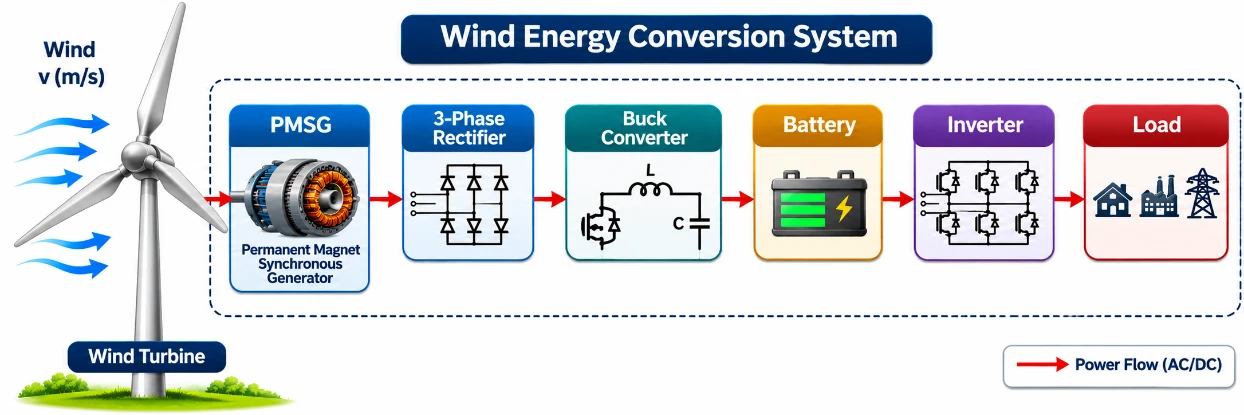
Fig. 1:Block diagram of the complete low-speed WPGP system.
Arduino/Proteus-based embedded power-control work. [16-18,22]
Motivated by this gap, the present study designs and evaluates, entirely through circuit-level simulation, a Mamdani FLC for PWM duty-cycle control of a three-phase synchronous MOSFET rectifier in a low-speed Wind Power Generation Plant (WPGP) prototype. The closed-loop performance of the controller is assessed through Proteus simulation across duty-cycle and input-voltage variations under both resistive and resistive–inductive loads, while the Arduino UNO, the IR2110 gate drivers, and the MOSFET bridge are implemented and exercised within the same Proteus circuit model, extending the kind of embedded, low-cost simulation reported in comparable Arduino/Proteus power-electronics studies.[16,17,22] The contributions of this study are threefold: (i) a Mamdani FLC design for three-phase synchronous-rectifier duty-cycle regulation, positioned against recent PI-versus-fuzzy and type-2/type-3 fuzzy comparisons on related converters;[14,24,25] (ii) a systematic, simulation-based characterization of how the duty cycle, input voltage, and load type jointly affect the output voltage and ripple in an inductor-less synchronous rectifier, including the ripple-plateau behavior noted above and left largely unaddressed in the classical rectifier-filtering literature;[19,21] and (iii) an explicit separation of controller performance from the structural voltage-conversion limits imposed by the topology and the available AC source, a distinction that recent low-speed and low-voltage WECS studies increasingly emphasize when a setpoint is not reached.[6,7,9] Given that the control method was limited to Type-1 fuzzy logic, all the data presented in this study are based solely on Proteus simulation results; full integration with the wind power plant unit was not achieved because of material constraints, necessitating independent testing using a three-phase AC source.
2. Materials and methods
2.1 System architecture and operating principles
The complete WPGP system comprises a Savonius-type wind turbine (0.8 m blade height, 13–15 kg, rated 800–1000 W) coupled to a 1000 W, 48 V three-phase permanent-magnet synchronous generator (PMSG); a three-phase PWM synchronous rectifier (the focus of this study); a buck converter stepping the rectified 48 VDC down to 27 VDC for battery charging; and a single-phase inverter supplying the load (Fig. 1), following the generator–rectifier–conditioning–load chain typical of low-speed PMSG-based WECS installations. [6,10]
Within the rectifier stage, the control objective is to keep the DC output close to a 48 V setpoint, matching the PMSG’s rated voltage. The signal path is as follows: three-phase AC source/generator → synchronous MOSFET rectifier → output filter capacitor → resistive (R) or resistive–inductive (R–L) load, with a voltage-sensing divider feeding the rectified output back to an Arduino UNO, which runs the Mamdani fuzzy logic controller (FLC) and issues the corrected PWM duty cycle to the three IR2110 gate drivers and, in turn, the six-switch MOSFET bridge. The controlled variable is therefore the rectified DC output voltage, and the manipulated variable is the PWM duty cycle applied to the bridge. A structural feature of the topology is the absence of a series filter inductor between the switched bridge and the output capacitor, a condition that is central to the ripple behavior analyzed in Section 3.4. Both purely resistive loads and resistive–inductive loads were used to exercise the rectifier, the latter representing the downstream single-phase inverter stage of the complete WPGP system, which is consistent with the closed-loop voltage-sensing feedback structure used in comparable PMSG-rectifier DVC designs.[13]
2.2 Three-Phase synchronous rectifier design
The 3-phase PWM rectifier consists of a PCB, MOSFET semiconductors, a capacitor filter, and control components comprising an Arduino UNO and a driver IC.
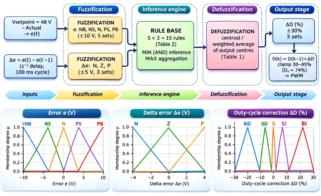
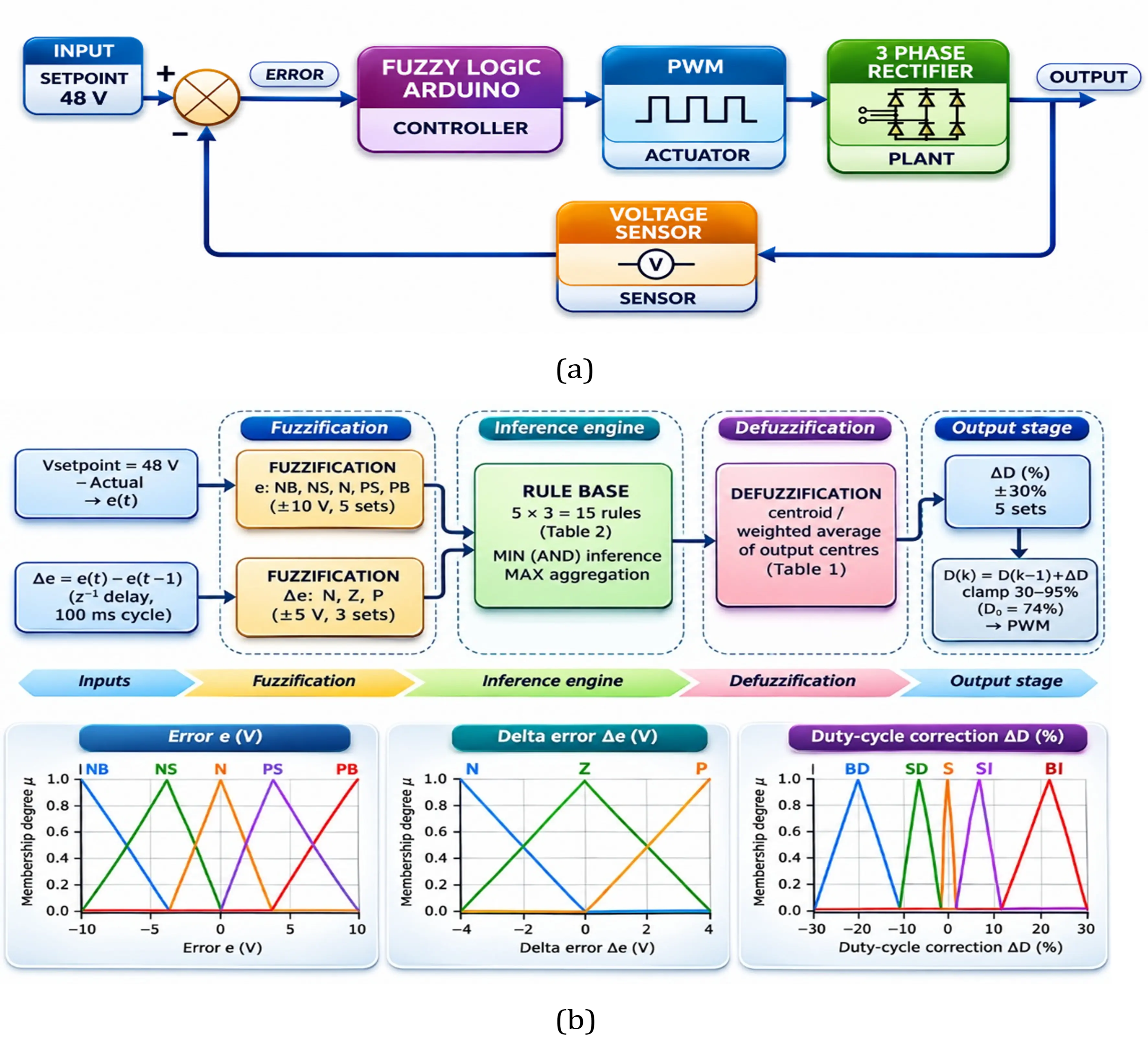
Fig. 2:Closed-loop control block diagram. (a) Closed-loop block diagram (upper panel); (b) architecture of the Mamdani FLC showing the inputs, fuzzification block, 5 × 3 rule base, defuzzification, and the membership functions of e, Δe, and ΔD (lower panel).
A MOSFET is a device controlled by a gate-source voltage to maintain conduction, characterized by very short switching times—ranging from tens to hundreds of nanoseconds.[30] The capacitor serves to eliminate the voltage ripple in the DC output caused by the sinusoidal current draw.[21] The PCB acts as an electromechanical platform that interconnects the electronic components.[15] The Arduino UNO is a microcontroller board programmed via the Arduino IDE using C/C++. [17] The IR2110 driver IC is a high-voltage, high-speed MOSFET/IGBT driver featuring independent high-side and low-side output channels capable of driving N-channel MOSFETs/IGBTs up to 500–600 volts in a high-side configuration.[18]. The rectifier stage uses six IRFP460 MOSFETs (500 V/20 A rating), providing a voltage and current margin above the PMSG’s 48 V, 1000 W nameplate rating arranged as a six-switch synchronous bridge, three IR2110 high/low-side gate-driver ICs with bootstrap circuits, and a 6800 μF/63 V output filter capacitor (sized from the target 6% ripple at 2000 W). Switching is generated by an Arduino UNO, which reads the rectified output through a 120 kΩ/10 kΩ voltage divider and issues 5 kHz, 120°-phase-shifted PWM signals (2 μs dead time) to the three gate-driver legs, with the MOSFET current rating, output-capacitor value, and interleg dead time size using standard switching-converter design practices.[19,30] The rectifier was exercised at AC input voltages of 48 V (the PMSG’s rated output) and 36 V (representing a reduced wind-speed condition) across three resistive loads (450, 650, and 1000 Ω) and three resistive–inductive loads (323, 645, and 1936 Ω).
2.3 Fuzzy logic controller (FLC) design
The closed-loop control structure (Fig. 2) compares the sensed rectifier output against a 48 V setpoint, matching
Table 1: Fuzzy rule base (15 rules)
| Error (e) \ Delta error (Δe) | Negative (N) | Zero (Z) | Positive (P) |
|---|---|---|---|
| Negative Big (NB) | BI | BI | SI |
| Negative Small (NS) | BI | SI | S |
| Neutral (N) | SI | S | SD |
| Positive Small (PS) | S | SD | BD |
| Positive Big (PB) | SD | BD | BD |
the generator's rated voltage, to obtain a voltage error, which the Arduino process with a Mamdani-type FLC to command the PWM duty cycle. The internal architecture of the FLC block is shown in Fig. 2(b): the voltage error e(t) and the delta error Δe are fuzzified with the membership functions plotted in the same figure, the 15 rules of Table 1 are evaluated with MIN inference and combined by MAX aggregation, and the aggregated result is defuzzified by the centroid (weighted-average) method to give the duty-cycle correction ΔD, which is added to the running duty cycle before it is applied as the PWM command.
The Mamdani method was selected over Sugeno, Tsukamoto, or type-2 fuzzy variants because its linguistic IF-THEN rules can be verified manually without an auxiliary consequent function, which is valuable for a system whose overall closed-loop behavior had not previously been characterized, which is consistent with reported comparisons showing that Mamdani inference is more transparent and easier to validate against expected control action than Sugeno-type systems in similar power-electronic control problems.[31] Two inputs are used, namely, the voltage error e(t), which is classified into five sets (negative Big, negative Small, neutral, positive Small, and positive Big) over ±10 V, given by e(t) = Vsetpoint - Vactual (1) and delta error Δe, classified into three sets (negative, zero, positive) over ±5 V, given by
Δe = e(t) - e(t-1) (2) where e(t−1) is the voltage error from the previous control cycle. The coarser 3-level resolution on Δe keeps the rule base to 5×3 = 15 rules rather than 25, limiting the computational load on the Arduino UNO for a 100 ms control cycle, while the finer 5-level output resolution and duty-cycle change ΔD, from Big Decrease to Big Increase over ±30%, allows large corrections far from the setpoint and fine corrections near it, since the output is added incrementally to the running duty cycle each cycle. Inference uses MIN/MAX composition with centroid (weighted-average) defuzzification, which is the standard combination for Mamdani-type controllers; the seed duty cycle is 74%.[31]
Membership functions: All the membership functions used for the error, delta-error, and duty-cycle-correction variables are triangular or trapezoidal; their linguistic sets and numerical ranges are summarized in Table 2. The triangular and trapezoidal membership functions are plotted in Fig. 2(b).
2.4 Fuzzy rule base and inference process
The complete 5×3 rule base, mapping the voltage error and delta error to the duty-cycle correction, is given in Table 1. For each control cycle, the firing strength of every rule is computed as the minimum of the two input membership degrees (MIN composition); the fifteen weighted contributions are then combined by a weighted average of their output centers (Table 2) to obtain the crisp duty-cycle correction, which is added to the running
Table 2: Fuzzy input and output linguistic sets used in the Mamdani FLC
| Variable | Set | Range |
|---|---|---|
| Voltage error, e (V) | Negative Big (NB) | −10 to −6 |
| Negative Small (NS) | −6 to −1 | |
| Neutral (N) | −1 to +1 | |
| Positive Small (PS) | +1 to +6 | |
| Positive Big (PB) | +6 to +10 | |
| Delta error, Δe (V) | Negative (N) | −5 to −1 |
| Zero (Z) | −1 to +1 | |
| Positive (P) | +1 to +5 | |
| Duty-cycle correction, ΔD (%) | Big Decrease (BD), center −20.5 | −30 to −10 |
| Small Decrease (SD), center −5.5 | −10 to −1 | |
| Stable (S), center 0.0 | −1 to +1 | |
| Small Increase (SI), center +5.5 | +1 to +10 | |
| Big Increase (BI), center +20.5 | +10 to +30 |
Table 3: Fuzzy rule-based verification in MATLAB (three representative test cases)
| Case | V(t) (V) | V(t−1) (V) | Error e | Delta error Δe | Output ΔD |
|---|---|---|---|---|---|
| Voltage drop | 45 | 48 | 3 | 3 | +22.4% (increase duty) |
| Voltage rise | 50 | 45 | −2 | −5 | −18.3% (decrease duty) |
| Voltage steady | 50 | 50 | −2 | 0 | −6.36% (decrease duty) |
duty cycle and clamped to the 30–95% safe operating range described in Section 2.3. Prior to being embedded in the circuit-level model, the rule base and defuzzification logic were sanity-checked in MATLAB at three representative operating points, summarized in Table 3, to confirm that the controller’s output direction and magnitude were physically sensible ahead of the closed-loop Proteus evaluation reported in Section 3.
2.5 Proteus simulation setup
To allow the simulation to be replicated, the Proteus model represented the three-phase AC source at 48 V (rated) and 36 V (reduced wind-speed condition), the six IRFP460 MOSFETs and three IR2110 gate drivers described in Section 2.2, and the 6800 μF output capacitor. The load bank comprised the same three resistive (450, 650, 1000 Ω) and three resistive–inductive (323, 645, 1936 Ω) conditions used in the simulation runs. The switching frequency (5 kHz), dead time (2 μs), and 30–95% duty-cycle clamp matched the Arduino firmware values. Two protocols were run: an open-loop duty-cycle sweep at a fixed VAC = 48 V with the duty cycle manually set to 30%, 50%, 74%, and 95% (Section 3.3) and a closed-loop fuzzy-control sweep with the 48 V setpoint held fixed at VAC = 48 V and 36 V (Section 3.5). Each condition was run until the output voltage and ripple waveform reached a repeating steady-state pattern before Vmax, Vmin, Vdc, and the ripple factor were recorded at the rectifier output/capacitor node.
3. Results and discussion
3.1 Proteus circuit-level implementation
The complete switching stage, comprising the Arduino UNO PWM generator, the three IR2110 high/low-side gate drivers with bootstrap circuits, and the six-switch IRFP460 MOSFET bridge, was implemented as a single Proteus schematic (Fig. 3) so that the fuzzy-corrected PWM duty cycle drives the switching bridge entirely within the simulation environment. The 5 kHz, 120°-phase-shifted switching pattern with a 2 μs dead time described in Section 2.2 was applied to the three gate-driver legs in this model, and the switching verification, open-loop, and closed-loop results reported in Sections 3.2–3.5 were obtained directly from this Proteus circuit.
The rectifier was exercised under two categories of load, matching the resistive and resistive–inductive conditions used throughout Sections 3.3–3.5. A resistive (R) load consists solely of a resistor, so the load current tracks every change in the applied voltage instantaneously and in phase. A resistive–inductive (R–L) load instead combines a series resistor and inductor; because the inductor opposes any abrupt change in current (v = L di/dt), the load current responds more gradually than the load voltage does and lags it in phase, which is representative of the downstream single-phase inverter stage that the rectifier ultimately supplies. Table 4 lists the three resistive and three resistive–inductive conditions used in the open-loop duty-cycle sweep, the input-voltage sweep, and the closed-loop fuzzy-control tests reported below.
Table 4: Resistive and resistive–inductive load conditions used in the rectifier tests
| Load type | Resistance/Impedance (Ω) |
|---|---|
| Resistive (R) | 450 |
| Resistive (R) | 650 |
| Resistive (R) | 1000 |
| Resistive–Inductive (R–L) | 323 |
| Resistive–Inductive (R–L) | 645 |
| Resistive–Inductive (R–L) | 1936 |
3.2 Proteus-based PWM and switching verification
Before evaluating the open-loop and closed-loop electrical performance of the rectifier, the switching stage itself, the Arduino UNO PWM generator, the three IR2110 gate-driver legs, and the six-switch MOSFET bridge, was checked block-by-block within the Proteus model to confirm that the PWM command issued by the Arduino UNO was correctly reproduced as complementary high-side (HO) and low-side (LO) gate signals before being applied to the power stage.
The representative HO/LO waveforms captured at the output of each of the three IR2110 gate drivers are shown in Fig. 4. Each panel spans three consecutive periods of the 5 kHz carrier (T = 200 μs), so the HO/LO pulses recur once per switching period; they are therefore PWM pulse trains rather than a single pulse, and the pulse width relative to T is the duty cycle commanded by the Arduino UNO. The corresponding reference PWM timings of one phase leg for duty cycles of 30, 50, 74, and 95% are shown in Fig. 4(d), in which HO and LO are complementary and separated by the 2 μs dead time, and the pulse width increases with the number of commanded duty cycles. In all three-phase legs, HO and LO are pulsed rather than sinusoidal, tracking the commanded PWM pattern, and no interval was found in which both outputs were simultaneously high; the brief low interval separating
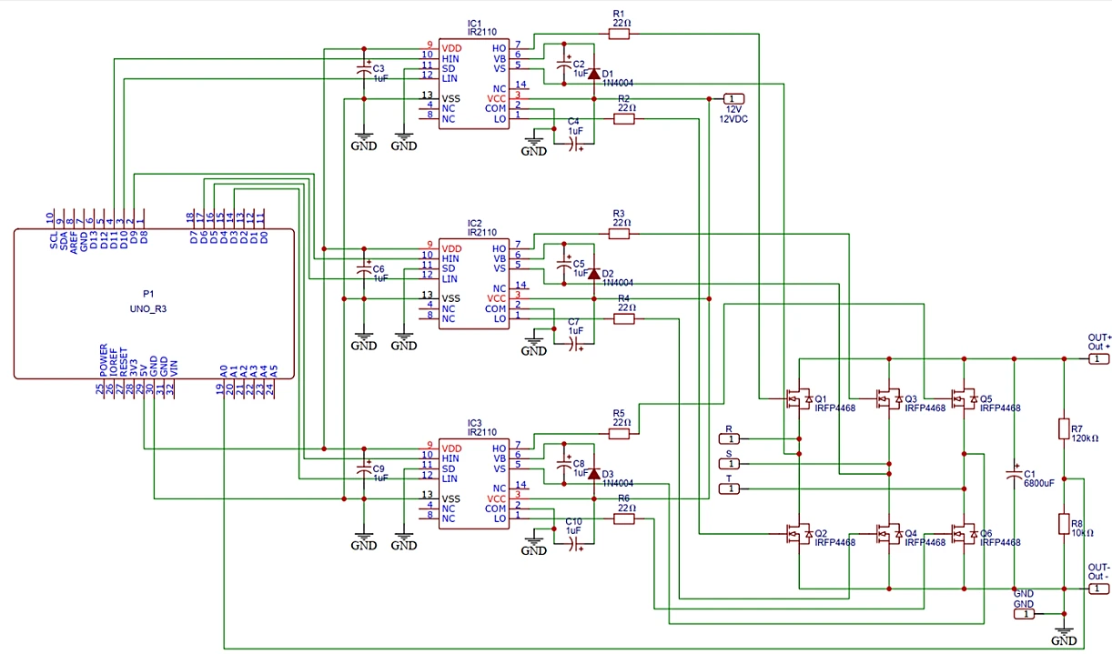
Fig. 3:Proteus schematic of the three-phase synchronous MOSFET rectifier circuit, including the gate-driver stage, output voltage/current meters, and resistive–inductive load branch.
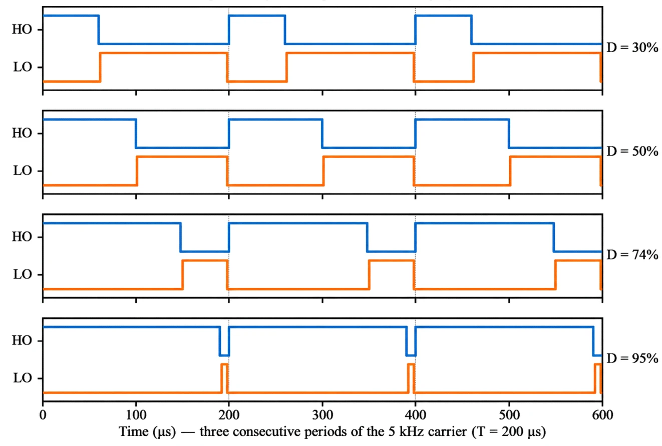
Fig. 4:Representative IR2110 gate-driver output waveforms (HO/LO) from Proteus switching verification: (a) phase leg A; (b) phase leg B; (c) phase leg C. (d) Reference PWM timing diagram of one phase leg (HO/LO) at duty cycles of 30, 50, 74 and 95%.
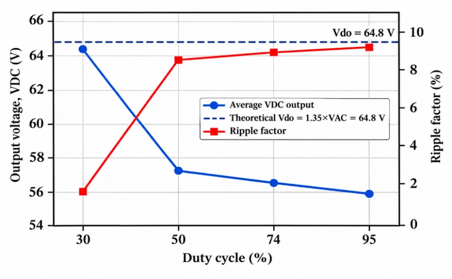
Fig. 5:Average output voltage and ripple factor versus duty cycle (VAC = 48 V)
Table 5: Effect of duty cycle variation on the rectifier output voltage (VAC = 48 V)
| Duty (%) | Vmax (V) | Vmin (V) | Vdc avg. (V) | Vdo theory (V) | Error vs. theory (%) |
|---|---|---|---|---|---|
| 30 | 66.1–66.4 | 61.4–62.9 | 64.4 | 64.8 | +0.5 to +2.5 |
| 50 | 65.6–66.2 | 47.8–49.8 | 57.3 | 64.8 | +1.2 to +2.2 |
| 74 | 65.0–65.8 | 46.7–48.8 | 56.5 | 64.8 | +0.3 to +1.5 |
| 95 | 64.7–65.8 | 46.0–48.0 | 55.9 | 64.8 | −0.2 to +1.5 |
each HO-to-LO and LO-to-HO transition corresponds to the 2 μs dead time specified in Section 2.2. Because no overshoot, was observed on any of the three legs, this simulated verification indicates that the IR2110 driver stage and its bootstrap circuit reproduce the intended dead-time behavior needed to prevent shoot-through in the MOSFET bridge, supporting the validity of the switching hardware model used to obtain the open-loop and closed-loop results reported in Sections 3.3–3.5.
3.3 Open-Loop characteristics under duty-cycle variation
Table 5 summarizes the effect of the duty cycle variation (at VAC = 48 V) on the output voltage, and Table 6 summarizes the corresponding ripple factor, which is averaged across the six load conditions. The average output voltage and ripple factor are plotted against the duty cycle in Fig. 5, where the dashed line indicates the theoretical output voltage Vdo.
The theoretical DC output limit of a three-phase full-wave rectifier is as follows:
Vdo = 1.35 × VAC (3)
At the rated input voltage (VAC = 48 V), Vdo = 1.35 × 48
= 64.8 V; the reference values are listed in the “Vdo theory” column of Table 5.
The ripple factor was computed as follows:
RippleRMS = (Vmax - Vmin)23 (4) then
Ripple(%) = RippleRMS(Vmax + Vmin)2 × 100% (5)
For example, at 50% duty on the 450 Ω load (Vmax = 66.2 V, Vmin = 49.8 V), Ripple RMS = (66.2 − 49.8)/(2√3) = 4.73 V, yielding a ripple factor of 4.73/58.0 = 8.2%, which is consistent with the values reported in Table 6.
As depicted in Fig. 5, the peak voltage remained essentially constant across all duty cycles (64.7–66.4 V) and close to the theoretical Vdo = 64.8 V, confirming that Vmax is set by the natural peak of the six-pulse rectified waveform rather than by the duty cycle itself. In contrast, Vmin decreases sharply as the number of duty cycles increases from 30% to 50% and then decreases only gradually to 95%, which drives the corresponding
Table 6: Effect of duty cycle variation on the ripple factor (VAC = 48 V; RF theory for an unfiltered 6-pulse rectifier = 4.2%)
| Duty (%) | Ripple p-p (V) | Ripple RMS (V) | Ripple factor (%) |
|---|---|---|---|
| 30 | 3.2–4.8 | 0.92–1.39 | 1.4–2.2 |
| 50 | 16.2–18.4 | 4.73–5.14 | 8.2–9.1 |
| 74 | 16.6–18.6 | 4.82–5.37 | 8.4–9.6 |
| 95 | 17.3–18.8 | 4.99–5.43 | 8.8–9.8 |
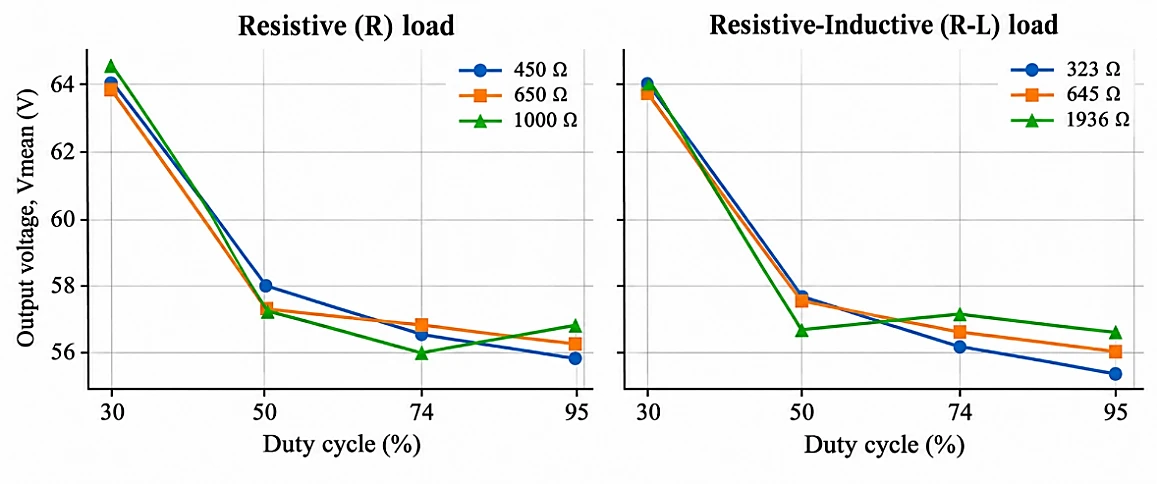
Fig. 6:Output voltage versus duty cycle, broken down by individual load: (a) resistive (R) loads; (b) resistive–inductive (R–L) loads.
decrease in average Vdc; therefore, the relationship between Vdc and the duty cycle is not the simple linear Vdc = D × Vdo expected of a buck-type converter; Vmax remains locked at the natural peak value of the rectifier, while the duty cycle determines how deeply Vmin is allowed to decrease during each switching cycle.
This trend is broken down by individual load, as shown in Fig. 6, which compares the three resistive (R) conditions against the three resistive–inductive (R–L) conditions. Both load types trace the same duty cycle dependence; the initial voltage decreases from 30% to 50% duty, followed by a shallow decline through 95%, and the R and R–L curves remain within approximately 1 V of each other at every duty cycle. This finding indicates that the output-voltage behavior is governed by the switching pattern and rectifier topology rather than by whether the load draws current resistively or through a series inductor.
3.4 Ripple-Plateau analysis
Ripple follows the same two-stage pattern: a sharp increase from 1.4–2.2% at 30% duty to a plateau of 8.2–9.8% from 50% to 95% duty, rather than the symmetric, D(1−D)-shaped ripple curve of a classical buck converter that would peak at D = 50% and decrease again toward D = 0% and 100%. This is consistent with the rectifier's topology, which has no series filter inductor: the output capacitor is exposed directly to the switched bus, so it charges quickly and then decays for a duration set by the switch's off-time within each 60° commutation window. As the duty cycle widens, the capacitor is allowed to decay for longer before recharging, increasing the ripple until the decay is instead bounded by the fixed 60° commutation window rather than by the duty cycle, resulting in the observed plateau. Because the ripple at a duty ≥50% is 4–6 percentage points above the theoretical six-pulse ceiling (~4.2%), the excess ripple originates from the interaction between the PWM conduction window and the natural six-pulse waveform, not from the rectification process itself. The same ripple-plateau pattern broken down by individual load is shown in Fig. 7. The resistive and resistive–inductive conditions increase from approximately 1.4–2.2% at 30% duty to the 8–10% plateau at a duty ≥50%, and the two load types remain interleaved rather than separating into distinct bands at any duty cycle. This confirms that the ripple mechanism described above is set by the capacitor's charge–discharge interaction with the PWM conduction window, not by the load's resistive or resistive–inductive character.
This transition is illustrated directly with representative Proteus oscilloscope traces from the same rectifier node
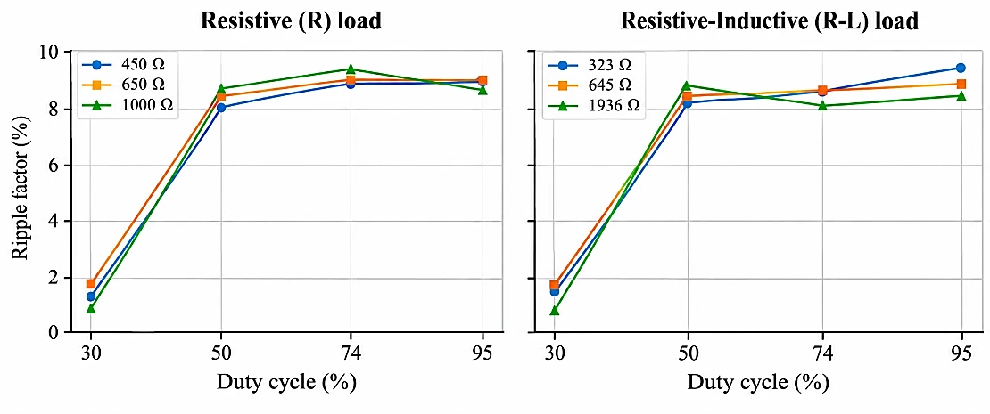
Fig. 7:Ripple factor versus duty cycle, broken down by individual load: (a) resistive (R) loads; (b) resistive–inductive (R–L) loads.
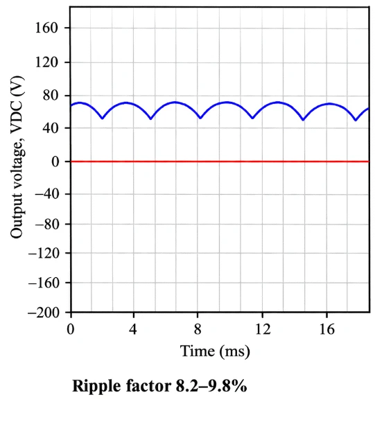
Fig. 8:Representative Proteus oscilloscope waveforms showing the ripple‒plateau transition: (a) low-ripple open-
loop condition at 30% duty; (b) high-ripple closed-loop steady state at VAC = 48 V. Horizontal axis: time (ms), 1 ms/div; vertical axis: output voltage (V), 20 V/div; the cyan line indicates the 0 V reference.
Table 7: Closed-loop fuzzy control performance at VAC = 48 V and 36 V
| VAC (V) | Vdo theory (V) | Vdc avg. (V) | Vmin/VAC ratio | Ripple factor avg. (%) |
|---|---|---|---|---|
| 48 | 64.80 | 64.94 | 0.984 | 9.2 |
| 36 | 48.60 | 46.79 | 0.988 | 7.9 |
(horizontal axis: time in ms; vertical axis: output voltage in V) in Fig. 8: Panel (a) shows the relatively flat output at 30% open-loop duty (ripple factor 1.4–2.2%), whereas Panel (b) shows the pronounced sawtooth-shaped ripple recorded once the closed-loop controller settles near its steady-state duty cycle at VAC = 48 V (ripple factor 8.2–9.8%). The visibly deeper and more frequent discharge notches in panel (b) are direct simulation evidence for the capacitor charge–discharge mechanism described above.
3.5 Closed-Loop FLC performance under input voltage variation
Table 7 compares the closed-loop fuzzy control performance at the two tested input voltages. The average output voltage and ripple factor at each input voltage are plotted in Fig. 9. The same theoretical relation applies at the reduced input voltage: Vdo = 1.35 × 36 = 48.6 V; the reference against which the VAC = 36 V row in Table 7 is compared.
Under closed-loop fuzzy control, the system regulated close to the 48 V setpoint at VAC = 48 V (Vmin/VAC = 0.984) but pushed the duty cycle toward its maximum at VAC = 36 V (Vmin/VAC = 0.988) because the theoretical ceiling at that input (Vdo = 48.6 V) leaves the controller no margin to reach 48 V through duty cycle adjustment alone; the fuzzy logic responded correctly to the available error signal in both cases. This finding indicates that the unmet setpoint at a low input voltage is a structural limitation of the inductor-less synchronous rectifier topology, not a fuzzy-controller design fault, since the peak voltage is fixed by the AC source (bridged through the MOSFET body diodes), whereas the minimum voltage is bounded by the fixed commutation window rather than by the duty cycle. Addressing this would likely require an explicit chopper/switching stage that separates the rectification and voltage-regulation
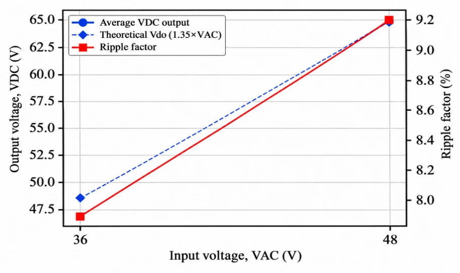
Fig. 9:Average output voltage and ripple factor versus input voltage VAC under closed-loop fuzzy control.
functions, for example, a series LC filter combined with a redesigned freewheeling scheme, rather than simply adding filter components to the existing switching arrangement.
4. Conclusion
In this study, a Mamdani-based fuzzy logic controller for PWM duty cycle regulation of a three-phase synchronous MOSFET rectifier intended for a low-speed wind power generation prototype was designed and evaluated using a Proteus circuit-level simulation with the rule base of the controller further sanity checked in MATLAB. In the complete switching stage, the Arduino UNO PWM generator, IR2110 gate drivers, and MOSFET rectifier bridge were implemented and exercised entirely within a Proteus circuit-level model, and a closed-loop Proteus simulation revealed that the fuzzy controller regulates the output voltage close to the 48 V setpoint when the input voltage permits it (VAC = 48 V) and otherwise saturates the duty cycle appropriately when the setpoint is structurally unreachable (VAC = 36 V). The peak output voltage tracked the theoretical six-pulse value (64.8 V) regardless of the duty cycle, whereas the ripple sharply increased from 1.4–2.2% at 30% duty to an 8.2–9.8% plateau at a duty ≥50%, which was attributed to the absence of a series filter inductor. These findings indicate that the observed setpoint shortfall reflects a structural limitation of the rectifier topology rather than a flaw in the fuzzy control design and point to the addition of a properly codesigned LC output filter as the most direct path to close the gap in future work.
Acknowledgment
The authors thank the Electrical Power Systems Study Program, Department of Electrical Engineering, State Polytechnic of Malang, for laboratory access and support during this research.
CRediT Author Contribution Statement
Ika Noer Syamsiana: Project administration, Supervision, Validation, Writing – Review & editing. Muhammad Akmal Nashiry: Conceptualization, Data curation, Formal analysis, Investigation, Methodology, Software, Visualization, Writing – Original draft. Harrij Mukti Khristiana: Supervision, Validation, Writing – Review & editing. Arwin Datumaya Wahyudi Sumari: Data Curation, Project Administration, Resources, Software. All authors have read and approved the final version of the manuscript for publication and agree to be accountable for all aspects of the work, ensuring that questions related to the accuracy or integrity of any part of the work are appropriately investigated and resolved.
Funding Declaration
This research did not receive any specific grant from funding agencies in the public, commercial, or not-for-profit sectors.
Data Availability Statement
The datasets generated and/or analyzed during the current study that support the findings are available from the corresponding author upon reasonable request.
Conflict of Interest
There is no conflict of interest.
Artificial Intelligence (AI) Use Disclosure
The authors declare that artificial intelligence (AI)-assisted tools were used only for language refinement, grammar improvement, and manuscript structuring purposes during the preparation of this work. All technical content, experimental implementation, results, and interpretations were independently developed and verified by the authors.
Supporting Information
Not applicable.
References
- [1] A. Lubis, Energi terbarukan dalam pembangunan berkelanjutan, Jurnal Teknologi Lingkungan BPPT, 2007, 8, 151118, doi: 10.29122/jtl.v8i2.420.
- [2] Kementerian ESDM, RUPTL PT PLN (Persero) tahun 2025–2034: Materi konferensi pers. Kementerian Energi dan Sumber Daya Mineral Republik Indonesia, 2025, https://jdih.esdm.go.id/dokumen/download?id=2025abskesdm188k.pdf.
- [3] N. A. Pambudi, D. K. Ulfa, I. R. Nanda, I. M. Gandidi, A. Wiyono, M. K. Biddinika, B. Rudiyanto, L. H. Saw, The future of wind power plants in Indonesia: Potential, challenges, and policies, Sustainability, 2025, 17, 1312, 2025, doi: 10.3390/su17031312.
- [4] Y. Tanoto, L. Diprasetya, N. Enano Jr., H. S. Warpindyasmoro, Utility-scale wind power generation potential in low-wind regions: Insights for achieving the sustainable energy transition in developing countries, International Journal of Renewable Energy Development, 2026, 15, 584–595, doi: 10.61435/ijred.2026.61756.
- [5] A. D. Cahyo, R. M. Fatwah, Utilization of a low-speed neodymium wind turbine generator as an alternative power source for homes in the North Cirebon coastal area, Indonesia, Malaysian Journal of Science and Advanced Technology, 2024, 4, 316–321, doi: 10.56532/mjsat.v4i3.352.
- [6] A. Alili, M. B. Camara, B. Dakyo, Vienna rectifier-based control of a PMSG wind turbine generator, Processes, 2022, 10, 413, doi: 10.3390/pr10020413.
- [7] M. A. Hannan, A. Q. Al-Shetwi, M. S. Mollik, P. J. Ker, M. Mannan, M. Mansor, H. M. K. Al-Masri, T. M. I. Mahlia, Wind energy conversions, controls, and applications: A review for sustainable technologies and directions, Sustainability, 2023, 15, 3986, doi: 10.3390/su15053986.
- [8] Y. K. Teklehaimanot, F. K. Akingbade, B. C. Ubochi, T. O. Ale, A review and comparative analysis of maximum power point tracking control algorithms for wind energy conversion systems, International Journal of Dynamics and Control, 2024, 12, 3494–3516, doi: 10.1007/s40435-024-01434-3.
- [9] W. K. Ntuli, M. Kabeya, K. Moloi, Review of low voltage ride-through capabilities in wind energy conversion systems, Energies, 2024, 17, 5321, doi: 10.3390/en17215321.
- [10] D. B. Tchoumtcha, C. T. Sanjong Dagang, G. Kenne, Synergetic control for stand-alone permanent magnet synchronous generator driven by variable wind turbine, International Journal of Dynamics and Control, 2024, 12, 2888–2902, doi: 10.1007/s40435-024-01384-w.
- [11] B. N. Reddy, R. Jalli, K. S. Prudhviraj, K. B. Shetty, C. R. Reddy, H. Kotb, A. Emara, M. Alruwaili, Wind turbine with line-side PMSG-fed DC-DC converter for voltage regulation, PLOS ONE, 2024, 19, e0305272, doi: 10.1371/journal.pone.0305272.
- [12] I. Batarseh, A. Harb, Uncontrolled Diode Rectifier Circuits. InPower Electronics: Circuit Analysis and Design, Cham: Springer International Publishing, 2017, 461-524, doi: 10.1007/978-3-319-68366-9_7.
- [13] [13] Y. Saidi, A. Mezouar, Y. Miloud, M. A. Benmahdjoub, M. Yahiaoui, Fuzzy logic based robust DVC design of PWM rectifier connected to a PMSG WECS under wind/load disturbance conditions, International Journal of Energetica, 2019, 4, 2543–3717.
- [14] R. Coteli, M. Uyar, A. Mohammadzadeh, Evaluation of dynamic response and power quality performance in type-3 fuzzy logic controlled PWM rectifiers, Electronics, 2026, 15, 1639, doi: 10.3390/electronics15081639.
- [15] F. Perdigones, J. M. Quero, Printed circuit boards: The layers’ functions for electronic and biomedical engineering, Micromachines, 2022, 13, 460, doi: 10.3390/mi13030460.
- [16] L. Cohen, J. B. Bernstein, I. Aharon, A bipolar current source resonant gate driver for GaN-driven SiC power devices, Electronics, 2025, 14, 224, doi: 10.3390/electronics14020224.
- [17] E. Pratidhina, H. Kuswanto, D. Rosana, Penggunaan Arduino Uno dan Common-Coding pada Percobaan Fisika Materi Kelistrikan, Cipta Media Nusantara, 2021.
- [18] International IOR Rectifier, IR2110(S)PbF/IR2113(S)PbF datasheet, https://www.infineon.com/assets/row/public/documents/24/49/infineon-ir2110-datasheet-en.pdf, Accessed 20 August 2026.
- [19] M. H. Rashid, Power electronics: Devices, circuits, and applications, 4th ed, Pearson, 2014.
- [20] Z. Zhou, J. Song, Y. Yu, Q. Xu, X. Zhou, Research on high-quality control technology for three-phase PWM rectifier, Electronics, 2023, 12, 2417, doi: 10.3390/electronics12112417.
- [21] S. Liao, P. Dourmashkin, J. W. Belcher, MIT physics 8.02: Electricity and magnetism. Massachusetts Institute of Technology, 2004.
- [22] M. Bathre, P. K. Das, Design and implementation of a fuzzy-logic-based hybrid power management system for self-powered wireless sensor nodes using Arduino Mega 2560 and Proteus, Journal of Energy Storage, 2024, 97, 112961, doi: 10.1016/j.est.2024.112961.
- [23] G. Nethaji, J. Kathirvelan, Hardware implementation and comparison of PID and fuzzy logic controllers for a DC-DC boost converter for renewable energy applications, Heliyon, 2024, 10, e36750, doi: 10.1016/j.heliyon.2024.e36750.
- [24] A. Daraz, A. Basit, G. Zhang, Performance analysis of PID controller and fuzzy logic controller for DC-DC boost converter, PLOS ONE, 2023, 18, e0281122, doi: 10.1371/journal.pone.0281122.
- [25] M. Bahgat, M. Ezzat, M. A. Attia, S. F. Mekhamer, N. M. Elbehairy, Comparative analysis of PI and fuzzy logic controller for grid connected wind turbine under normal and fault conditions, Scientific Reports, 2025, 15, 1954, doi: 10.1038/s41598-024-85073-w.
- [26] Y. Saidi, A. Mezouar, Y. Miloud, M. A. Benmahdjoub, A Robust Control Strategy for Three Phase Voltage t Source PWM Rectifier Connected to a PMSG Wind Energy Conversion System, 2018 International Conference on Electrical Sciences and Technologies in Maghreb (CISTEM), Algiers, Algeria, 2018, 1-6, doi: 10.1109/CISTEM.2018.8613359.
- [27] A. Taibi, K. Hartani, T. M. Chikouche, N. Aouadj, Fuzzy logic-based DPC for PWM rectifiers: Enhancing power quality and advancing the sustainable development goals, Journal of Lifestyle and SDGs Review, 2025, 5, e06118, doi: 10.47172/2965-730X.SDGsReview.v5.n04.pe06118.
- [28] K. N. Khallouf, Z. Laid, H. Benbouhenni, N. Debdouche, Z. M. S. Elbarbary, Adaptive fuzzy logic control for microgrid-connected hybrid photovoltaic/wind generation systems, Energy Reports, 2024, 12, 4741–4756, doi: 10.1016/j.egyr.2024.10.042.
- [29] S. Karthikeyan, C. Ramakrishnan, A hybrid fuzzy logic-based MPPT algorithm for PMSG-based variable speed wind energy conversion system on a smart grid, Energy Storage and Saving, 2024, 3, 295–304, doi: 10.1016/j.enss.2024.08.001.
- [30] N. Mohan, T. M. Undeland, W. P. Robbins, Power electronics: Converters, applications, and design, 2nd ed. John Wiley & Sons, 1995.
- [31] T. Samavat, M. Nazari, M. Ghalehnoie, M. Azimi Nasab, M. Zand, P. Sanjeevikumar, B. Khan, A comparative analysis of the Mamdani and Sugeno fuzzy inference systems for MPPT of an islanded PV system, International Journal of Energy Research, 2023, 2023, 7676113, doi: 10.1155/2023/7676113.
Publisher Note
Publisher Note: The views, statements, and data in all publications solely belong to the authors and contributors. GR Scholastic is not responsible for any injury resulting from the ideas, methods, or products mentioned. GR Scholastic remains neutral regarding jurisdictional claims in published maps and institutional affiliations.
Open Access
This article is licensed under a Creative Commons Attribution-NonCommercial 4.0 International License, which permits the non-commercial use, sharing, adaptation, distribution and reproduction in any medium or format, as long as appropriate credit to the original author(s) and the source is given by providing a link to the Creative Commons License and changes need to be indicated if there are any. The images or other third-party material in this article are included in the article's Creative Commons License, unless indicated otherwise in a credit line to the material. If material is not included in the article's Creative Commons License and your intended use is not permitted by statutory regulation or exceeds the permitted use, you will need to obtain permission directly from the copyright holder. To view a copy of this License, visit: https://creativecommons.org/licenses/by-nc/4.0/
© The Author(s) 2026